After having introduced the bases de l’acoustique, we will focus in this article on the radiation of acoustic energy. We will see how to use the already established acoustics formulas to calculate the sound intensity generated by a vibrating solid. We will focus on the three cases that we will need to understand, later, the acoustic radiation of a loudspeaker: the pulsing sphere, the acoustic dipole, and the encased piston.
Pulsing sphere model
Description
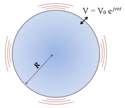
The source considered here is a solid sphere of radius R whose surface oscillates at the uniform speed \underline{V} = V_0 \exp{(j \omega t)}. The amplitude of the oscillations is assumed to be small compared to the radius R. The air pressure is thus disturbed and a sine sound wave is emitted.

The symmetry of the problem indicates that the acoustic quantities depend only on time and distance r to the source. Hence the sound waves emitted by the pulsing sphere are spherical.
Acoustic pressure and velocity
The corresponding formulas in the case of spherical waves are :
\displaystyle{ \underline{p} = \frac{\underline{A}}{r} \exp{ \left[ j(\omega t - kr) \right] } }
\displaystyle{ \underline{u}_r = \left( 1 - \frac{j}{kr}\right) \frac{\underline{p}}{\rho_0 c} }
At the interface between the sphere and the air, the velocity of the air is equal to that of the surface of the sphere. The constant \underline{A} can therefore be determined. Let's inject the expression of the pressure into that of the velocity for r = R, et égalisons avec l’expression de la vitesse de la surface de la sphère :
\displaystyle{ \underline{u}_r (R) = \left( 1 - \frac{j}{kR}\right) \frac{\underline{A}}{\rho_0 c R} \exp{ \left[ j(\omega t - kR)\right] } = V_0 \exp{(j\omega t)} }
We get:
\displaystyle{ \underline{A} = \rho_0 c R V_0 \frac{ \exp{(jkR)} }{1-\frac{j}{kR}} = j \omega \rho_0 R^2 V_0 \frac{ \exp{(jkR)} }{1 + jkR} }
Note that this "constant" depends on the vibration frequency of the source!
The acoustic pressure is then:
\displaystyle{ \underline{p} = j \omega \rho_0 R^2 V_0 \frac{\exp{(jkR)} }{1 + jkR} \frac{\exp{ \left[ j(\omega t - kr) \right] }}{r} }
Now we define the acoustic flow Q of the source as the volume displaced by its vibrations per unit time: Q = Q_0 \exp{(j\omega t)} = 4 \pi R^2 V . The expression of \underline{p} becomes:
\displaystyle{ \underline{p} = \frac{ j \omega \rho_0 Q_0}{4\pi} \cdot \frac{\exp{(jkR)}}{1 + jkR} \cdot \frac{\exp{ \left[ j(\omega t - kr) \right] }}{r} }
As for the acoustic speed \underline{u}:
\displaystyle{ \underline{u}_r = \left( 1 - \frac{j}{kr}\right) \frac{ j \omega Q_0}{4\pi c} \cdot \frac{\exp{(jkR)}}{1 + jkR} \cdot \frac{\exp{ \left[ j(\omega t - kr) \right] }}{r} = \left( 1 + jkr \right) \frac{ Q_0}{4\pi} \cdot \frac{\exp{(jkR)}}{1 + jkR} \cdot \frac{\exp{ \left[ j(\omega t - kr) \right] }}{r^2}}
The acoustic monopole
It is difficult to design a loudspeaker whose membrane is a sphere, and one could doubt the importance of the previous calculation ... However, the model of the pulsating sphere will be of great use to us for the following two reasons:
- When the wavelengths are large compared to the dimensions of the speaker, it is experimentally verified that the acoustic radiation produced is very close to that of a pulsating sphere. The pulsating sphere is therefore a good model for the bass of an enclosure, even if only a part of the surface of the sphere vibrates. For the dimensions of the radios we use, about 50 cm, we can describe correctly by this model wavelengths greater than 1.5m, which corresponds roughly to frequencies below 200 Hz.
- Finally, by virtue of the Huygens-Fresnel principle, a complex vibrating source (the membrane of a loudspeaker) can be described below by considering it as a sum of spherical elementary sources.
Note that, in these two applications, the dimensions R of the source are small (relatively for the first, infinitesimal for the second). We can therefore simplify the expressions by making the radius of the sphere tend towards zero to obtain the expressions of the acoustic monopole :
\displaystyle{ \boxed{ \underline{p} = \frac{ j \omega \rho_0 Q_0}{4\pi} \cdot \frac{\exp{ \left[ j(\omega t - kr) \right] }}{r} }}\displaystyle{\underline{u}_r = \left( 1 + jkr \right) \frac{ Q_0}{4\pi} \cdot \frac{\exp{ \left[ j(\omega t - kr) \right] }}{r^2}}Sound intensity and level
We have already shown that, for a spherical wave : \displaystyle{ I = \frac{p_\text{eff}^2}{\rho_0 c}}
Thus, the sound intensity of the wave produced by an acoustic monopole is :
\displaystyle{\boxed{ I = \frac{\rho_0 }{2c} \left( \frac{ \omega Q_0}{4\pi r} \right)^2 } }
As we have already mentioned when discussing geometric attenuation, the sound intensity decreases as the square of the distance to the source. The emitted energy is diluted over an area that increases as the square of the distance.
The sound level generated by the monopole results from this:
L(r) = 10 \log{ \frac{I(r)}{I_0} } = 10 \log{ \left[ \frac{\rho_0 }{2 I_0 c} \left( \frac{ \omega Q_0}{4\pi r} \right)^2 \right]} = 10 \log{ \left( \frac{\rho_0 }{32 \pi^2 I_0 c}\right) + 20 \log \left( \frac{ \omega Q_0}{r} \right)}
where, after the last equality, the only variable quantities are grouped in the last term.
Finally, the acoustic power \mathcal{P}_\text{s} émise par la source est calculable en sommant l’intensité sonore sur une sphére centrée sur la source de rayon r\prime :
\mathcal{P}_\text{ac} = 4\pi r\prime^2 I(r\prime) \iff \displaystyle{\boxed{ \mathcal{P}_\text{ac} = \frac{\rho_0 }{8\pi c} \left( \omega Q_0\right)^2 }}
Radiation's impedance
Formula
Let's go back to the pulsating sphere of radius R . By vibrating, it generates pressure variations in the air in its vicinity. These pressure variations generate, in turn, a force on the surface of the source. There is thus a phenomenon of coupling between the source and the environment it disturbs.
This force is naturally written : \underline{f} = - \underline{p}(R) \cdot S
where S = 4 \pi R^2 is the surface of the pulsating sphere, and where the negative sign comes from the fact that the force exerted by the air is directed towards decreasing r .
We showed that:
\displaystyle{ \underline{p}(R) = j \omega \rho_0 R^2 V_0 \frac{\exp{(jkR)} }{1 + jkR} \frac{\exp{ \left[ j(\omega t - kR) \right] }}{R} = \rho_0 R j \omega V_0 \exp{ (j\omega t)} \frac{1 }{1 + jkR}}We have seen that the model of the pulsating sphere was valid only at low frequencies, that is kR \ll 1At first order it yields: \left( 1 + jkR \right)^{-1} \approx 1 - jkR :
\displaystyle{ \underline{p}(R) \approx \rho_0 R (1 - jkR) j \omega V_0 \exp{ (j\omega t)} = \rho_0 (1-jkR) j \omega \underline{V} = \left[ \frac{\rho R \omega^2}{c} + j \omega \rho_0 R \right] \underline{V} }The force exerted by the air on the vibrating structure is thus:
\underline{f} = \left[- \frac{\rho R S \omega^2}{c} - j \omega \rho_0 R S \right] \underline{V}
We define theradiation impedance Z_{\text{ray}} as the ratio of the force \underline{f}\prime = -\underline{f} exerted by the vibrating surface on the air and the acoustic velocity \underline{u}(R) = \underline{V}(R) generated in the process:
\displaystyle{ Z_{\text{R}} = \frac{-\underline{f}}{\underline{u}} = \frac{\rho R S \omega^2}{c} + j \omega \rho_0 R S}
This quantity expresses the resistance of the air to vibrate under the action of the force.
Radiation's mass and resistance
Finally, we note that j \omega V_0 \exp{ (j\omega t)} corresponds to the acceleration \underline{a} of a point on the vibrating surface, so that the force can be written :
\displaystyle{ \underline{f} \approx -\rho_0 R S \underline{a} - \frac{\rho_0 R^2 \omega^2 S}{c} \underline{V} }
The coefficient \rho_0 R S of the acceleration is homogeneous to a mass that we will call radiation mass m_\text{R}. The second term is a fluid friction force of the type -R_\text{R} \underline{V}. R_\text{R} = \frac{\rho_0 R^2 \omega^2 S}{c} is the radiation resistance.
Thus, when we look for the equation of motion of the mobile part of a loudspeaker, Newton's second law will be written :
m \underline{a} = \Sigma \left(\text{autres forces}\right) + \underline{f}
\iff (m + m_\text{R}) \underline{a} = \Sigma \left(\text{autres forces}\right) - R_\text{R} \underline{V}
The radiation mass is interpreted as a mass of air moving along with the vibrating source. The radiation resistance is the friction coefficient translating the conversion of mechanical energy into acoustic energy: it explains the acoustic radiation of the structure.
With these notations, the radiation impedance is written :
\displaystyle{ \boxed{ Z_{\text{R}} = R_\text{R} + j \omega \, m_\text{R} }}
where
\displaystyle{R_\text{R} = \frac{\rho_0 S^2\omega^2 }{4\pi c} } \hspace{2cm}m_\text{R}= \rho_0 \frac{S^{3/2}}{2\sqrt{\pi}}
If the radiation mass of the pulsating sphere is kind enough to be a constant it is not the same for the radiation resistance which varies as the square of the pulsation. We can see from its expression that the conversion of mechanical energy of vibration of the source into acoustic energy will be very poor at low frequencies. Let's see this in detail.
Radiation factor
The radiation factor \sigma quantifies the efficiency of the conversion of mechanical energy of vibration into acoustic energy. It is defined by the relationship :
\displaystyle{ \boxed{ \sigma = \frac{\mathcal P_\text{ac}}{\rho_0 c S V_\text{eff}^2} }}
where the denominator corresponds to the acoustic power of the plane wave generated by an infinite plane vibrating at the same speed, measured on a surface equal to that of the source. Now, for the pulsating sphere, we have seen above that :
\displaystyle{ \mathcal{P}_\text{ac} =\frac{\rho_0 \omega^2 S^2 V_0^2}{8\pi c} }
Hence, the radiation factor of a pulsating sphere is :
\displaystyle{ \sigma = \frac{S \omega^2}{4\pi c^2} = R^2 k^2 }
The efficiency of the power transfer therefore varies as the square of the pulsation: it will be low in the bass, as has already been pointed out.
Note that the acoustic resistance can be written as a function of the radiation factor:
R_\text{R} = \rho_0 c S \sigma
An important fact should be noted here. Only one characteristic of the loudspeaker plays a role in the acoustic resistance and the radiation factor: its diameter (and therefore its surface). In terms of the efficiency of the transfer of mechanical energy from vibration to acoustic energy, the diameter of the loudspeaker is therefore the only factor that can be influenced.
To compensate for low transfer efficiency with a small loudspeaker, some manufacturers propose to increase the speed at which the membrane vibrates. For the same frequency of vibration, this consists in increasing the excursion of the loudspeaker membrane. But it is important to see that, in the formula giving the acoustic power, the surface is squared and therefore the diameter is to the power four: to obtain the same power with a loudspeaker of half the diameter, it would be necessary to increase the maximum excursion by a factor of four. If we look at the characteristics of "large excursion" loudspeakers, we realize that they are far from being able to compete with large loudspeakers in terms of bass reproduction.
Radiated acoustic power
We can now find the expression of the emitted power from the previous results. The fluid friction force -R_\text{R}\underline{V} described by the radiation resistance is responsible for the emission of acoustic waves.
The sound power is obtained by taking the scalar product of the force exerted by the source on the air with the speed of the air at the interface, its average is therefore :
\displaystyle{ \mathcal{P}_\text{ac} = \frac{1}{T} \, \int_0^T \Re(R_\text{R}\underline{V})\, \Re(\underline{V} )\text{d}t = R_\text{R}\frac{1}{T} \, \int_0^T \Re(\underline{V}\,\underline{V}^*) \text{d}t = R_\text{R} \frac{V_0^2}{2} }
That is:
\boxed{\mathcal{P}_\text{ac} = R_\text{R}V_\text{eff}^2 }
By sloting in the expression of the radiation resistance, we find the expression already calculated above:
\displaystyle{ \mathcal{P}_\text{ac} = \frac{\rho_0 R^2 \omega^2 S}{c}\frac{V_0^2}{2} = \frac{\rho_0 }{8\pi c} \left( \omega Q_0\right)^2 }
Acoustic dipole
Description
We get an acoustic dipole by placing at a short distance L \ll \lambda from each other two monopoles vibrating in phase opposition. We see here the interest of the modeling in this blog: when the membrane of a loudspeaker moves to the right, it generates an overpressure on the right and a depression on the left. A loudspeaker not mounted in a box behaves like a dipole.

The beautiful and simple spherical symmetry of the monopole is thus replaced by a cylindrical symmetry: the physical quantities will depend here, in addition to the coordinate r, of the coordinate \theta.
The two sources in phase opposition will generate interference. In particular, we can already see that, if the observer is placed at \theta = \frac{\pi}{2}, she will receive at the same time the opposite contributions of the two monopoles: the sound intensity will be zero.
Before going into details, let's see the dramatic consequences in terms of bass for the speakers. In order for the sound pressure to be maximal, let's place the observer on the axis y. For large wavelengths, the path difference between the two waves will be weak: the acoustic waves generated by the two monopoles will cancel almost entirely. The example below shows the result of this superposition for a wave of frequency f = 50 \,\text{Hz} and a distance L = 5 \, \text{cm}. The dotted curves indicate the pressure that would be observed with each monopole emitting alone, the green curve is the result of the superposition of the acoustic waves.

The sound pressure is divided by 20 between the monopole and the dipole in this example: the sound level produced by the dipole is therefore 20 \,\log 20 = 26 \text{dB} below that produced by a monopole of the same acoustic flow!
Acoustic pressure
Let's call Q_+ = Q_0 \exp{(j \omega t)} and Q_- = -Q_0 \exp{(j \omega t)} the acoustic flows of the two sources, which are opposite since they vibrate in phase opposition. The acoustic pressure obtained is of course the sum of the acoustic pressures coming from each of the monopoles:
\displaystyle{ \underline{p} = \underline{p}_+ + \underline{p}_- = \frac{ j \omega \rho_0 Q_+}{4\pi} \cdot \frac{\exp{ \left[-j kr_+ \right] }}{r_+} + \frac{ j \omega \rho_0 Q_-}{4\pi} \cdot \frac{\exp{ \left[ - j kr_- \right] }}{r_-} }
\displaystyle{ \iff \underline{p} = \frac{ j \omega \rho_0 Q_0}{4\pi} \cdot \left( \frac{\exp{ \left[- jkr_+ \right] }}{r_+} - \frac{\exp{ \left[ -jkr_- \right] }}{r_-} \right) \exp{(j \omega t)} }
We have r_+ and r_- close to r, therefore let's perform a Taylor expansion of the term in parentheses:
\frac{\exp (- jkr_+ ) }{r_+} \approx \frac{\exp (- jkr) }{r} + (r_+ - r) \frac{ \partial}{ \partial r} \left( \frac{\exp{(-jkr_+)}}{r_+}\right)_{r_+=r}
\iff \frac{\exp (- jkr_+ ) }{r_+} \approx \frac{\exp (- jkr) }{r} + (r_+ - r) (-\frac{1}{r}-jk) \frac{\exp{(-jkr)}}{r}
The same is done for the term containing the r_-, and we get:
\frac{\exp{ \left[- jkr_+ \right] }}{r_+} - \frac{\exp{ \left[ -jkr_- \right] }}{r_-} \approx (r_+ - r_-) (-\frac{1}{r^2}-\frac{jk}{r}) \exp (-jkr)
Let us now express r_+ -r_- using the diagram below and the good old Pythagorean theorem.

With (x,\,y) the Cartesian coodinates of the point Md’observation :
r_+^2 - r_-^2 = \left( x^2 + \left( y + \frac{L}{2}\right)^2\right) - \left( x^2 + \left( y - \frac{L}{2}\right)^2\right) = 2Ly = 2L r \cos \theta
Furthermore: r_+^2 - r_-^2 = (r_+ - r_-)(r_+ + r_-) \approx 2r(r_+ - r_-) d’où r_+ - r_- \approx L \cos \theta.
It comes then for the sound pressure :
\displaystyle{ \underline{p} = -\frac{ j \omega \rho_0 Q_0}{4\pi} \cdot L \cos \theta \left(\frac{1}{r^2}+\frac{jk}{r}\right) \exp (-jkr) \exp{(j \omega t)} }
That is:
\displaystyle{\boxed{ \underline{p} = \frac{ k^2 \rho_0 c L Q_0}{4\pi r} \, \cos \theta \, \left(1 + \frac{1}{jkr}\right) \exp [j(\omega t - kr)] }}
Unlike the radiation of the monopole, two terms appear here: one in 1/r^2 dominant in the near field (kr \gg 1), and one in 1/r dominant in the far field (kr \ll 1). The limit defining the far field depends of course on the frequency. But, for a typical listening distance of 3m, at 40 Hz :
kr = \frac{\omega}{c}r = \frac{2 \pi f}{c}r = \frac{2 \pi \times 40}{343}\times 3 = 2,19 > 1
The contribution of the near field will thus be weak for the low frequencies and totally negligible for the high frequencies: we are more interested in the far field for which
\displaystyle{ \underline{p}_\text{CL} = \frac{ k^2 \rho_0 c L Q_0}{4\pi r} \, \cos \theta \, \exp [j(\omega t - kr)] }
Acoustic velocity
We start as usual with the linearized Euler equation:
\displaystyle{\rho_0 j \omega\cdot \vec{\underline{u}} = - \vec{\nabla}\underline{p} }
with, in cylindrical coordinates, \vec{\nabla} = \frac{\partial}{\partial r} \vec{e}_r + \frac{1}{r}\frac{\partial}{\partial \theta} \vec{e}_\theta.
The radial coordinate is:
\displaystyle{ \underline{u}_r = -\frac{1}{j \omega \rho_0} \frac{\partial}{\partial r}\underline{p} }
\displaystyle{ \iff \underline{u}_r = \frac{k^2 Q_0 L}{4\pi r} \cos \theta \left( 1 + \frac{2}{jkr} - \frac{2}{(kr)^2} \right) \exp \left[j(\omega t - kr)\right] }
The orthoradial \theta coordinate is:
\displaystyle{ \underline{u}_\theta = -\frac{1}{j \omega r \rho_0} \frac{\partial}{\partial \theta}\underline{p} }\displaystyle{ \iff \underline{u}_\theta = \frac{j k Q_0 L}{4\pi r^2} \sin \theta \left( 1 + \frac{1}{ jkr} \right) \exp \left[j(\omega t - kr)\right] } .
Sound intensity
Only the radial coordinate of the acoustic velocity is to be taken into account in the calculation, since the sound intensity corresponds to the power crossing a unit surface orthogonal to the direction of propagation of the wave. All calculations done, we obtain :
\displaystyle{ I = \frac{1}{2} \Re (\underline{p}\,\underline{u}_r^*) = \frac{\rho_0}{2c^3} \left( \frac{\omega^2 L Q_0}{4\pi r} \right)^2 \cos^2 \theta }The sound level is deduced as usual:
L = 10 \, \log\left(\frac{I}{I_0}\right)
The radiation diagram of an acoustic dipole is shown below:

The dipole is aligned on the vertical axis, as in the previous figures.
The sound level is represented, the concentric circles give the levels at +18, -3, -18 and -36 dB.
The level drops by 3dB around 45°: the sound intensity is then divided by two.
Acoustic power
It is obtained by integration of the sound intensity on a sphere centered on the origin, the surface element in spherical coordinates being : \text{d}S = \sin(\theta) r^2 \text{d}\theta \text{d}\phi :
\mathcal{P}_ \text{ac} = \int_0^{2\pi} \int_0^{\pi} I(r) \sin(\theta) r^2 \text{d}\theta \text{d}\phi
\iff \mathcal{P}_ \text{ac} = \frac{\rho_0c}{16 \pi} \left(k^2LQ_0 \right)^2 \int_0^{\pi} \cos^2 (\theta) \sin(\theta) \text{d}\theta
\iff \boxed{ \mathcal{P}_ \text{ac} = \frac{\rho_0 c \omega^4}{24 \pi c^3} \left(LQ_0 \right)^2 }
It depends, like the acoustic intensity, on the power 4 of the pulse, while the expression of the acoustic power for the monopole varied as \omega^2.
Comparing the two expressions, at identical acoustic flows leads to :
\displaystyle{ \frac{\mathcal{P}_\text{monopôle}}{\mathcal{P}_\text{dipôle}} = \frac{3}{(kL)^2}}
At low frequencies, this ratio is large: the dipole is much less efficient than the monopole to transfer its energy to the air. This result was already clearly visible on the radiation diagram.
This is due, as we have already said, to the destructive interference between the two sound waves. For an unmounted loudspeaker, which therefore behaves like a dipole, we speak of acoustic short circuit to describe this phenomenon of significant reduction of the power in the low frequencies: we can see the need to insert the speaker in a cabinet to suppress the rear wave. We will come back to this in an article on enclosed speakers.
The baffled circular piston
Description
We will establish here a model of the radiation of a loudspeaker membrane. In order to get rid of the back wave and the associated acoustic short circuit, the membrane will be considered embedded in an infinite (y,\, z) plane. Loudspeaker manufacturers will say that the speaker is baffled.
The membrane itself will be modeled as a circular piston of radius a and surface S=\pi a^2 and will as such be considered as flat and non-deformable. In this way, all the points of the membrane will have the same speed \vec{\underline{V}}(t) = V_0 \exp(j\omega t) and will therefore vibrate in phase.
Finally, we will limit ourselves to the calculation in far field: we will suppose kr \gg 1.
The situation being symmetrical by rotation around the (Oy)axis, it will be enough to calculate the acoustic quantities measured by observers M located in the (y, \,z)plane, and whose polar coordinates are M(r, \,\theta).
The model is summarized in the following diagram:

We will discuss the limitations of this modeling at the end of the section.
Huygens-Fresnel principle
We have here to calculate the acoustic quantities due to an extended source. The approach to tackle such a problem is the same as in optics when studying diffraction. The Huygens-Fresnel principle states that an extended source of surface S can be decomposed into spherical elementary sources of elementary surfaces \text{d}S. Acoustic quantities measured in M will be the sum of the contributions of these elementary sources.
We already have an elementary spherical source: it is obviously the acoustic monopole. However, a subtlety is introduced here. The monopoles emit on the supposedly perfectly rigid surface of the piston: the wave emitted towards the half-space y<0 is therefore reflected towards the front of the membrane. Thus, the acoustic pressure and velocity measured at the front of the membrane will be twice as important, while they will be null at the back.
The formula for sound pressure established at the beginning of the article becomes :
\displaystyle{ \underline{p} = \frac{ j \omega \rho_0 V_0\text{d}S}{2\pi} \cdot \frac{\exp{ \left[ j(\omega t - kr) \right] }}{r} }
Acoustic pressure

We thus have to integrate at observation point M the set of contributions of the elementary sources identified by their polar coordinates (\mathcal{l}, \, \psi) in the plane (x, \, z) :
\displaystyle{ \underline{p} = \frac{ j \omega \rho_0 V_0}{2\pi} \exp ( j\omega t) \int_0^{2\pi} \int_0^a \frac{\exp (- j k u)}{u} l\text{d}l \text{d}\psi }
In the far field approximation, M is at infinity, \vec{u} and \vec{r} are thus almost collinear. The figure below represents the plane containing the origin, M and \text{d}S , it allows us to see that u \approx r - l \cos \delta.

In addition, the relationships of spherical trigonometry let us write: \cos \delta = \cos \theta \cos \psi. The formula for pressure becomes:
\displaystyle{ \underline{p} = \frac{ j \omega \rho_0 V_0}{2\pi} \frac{\exp \left[ j(\omega t- kr)\right] }{r} \int_0^{2\pi} \int_0^a \exp ( j k l \cos \theta \cos \psi) l\text{d}l \text{d}\psi }\iff \displaystyle{ \underline{p} = \frac{ j \omega \rho_0 V_0}{2\pi} \frac{\exp \left[ j(\omega t- kr)\right] }{r} \int_0^a l \left( \int_0^{2\pi} \exp ( j k l \cos \theta \cos \psi) \text{d}\psi \right) \text{d}l }
We just stumble across Bessel functions J_n regularly encountered in physics in problems with cylindrical symmetry, and whose results are known:
\left\{ \begin{array}{ll} J_0(X) = \frac{1}{2\pi} \int_0^{2\pi} \exp (j X \cos \psi) \text{d}\psi \\ J_1(X) = \frac{1}{X} \int_0^X u \, J_0(u) \text{d}u \end{array} \right.
The double integral becomes:
2\pi \int_0^a l J_0 \left(kl\cos\theta\right) \text{d}l
Then, by labeling u = kl\cos\theta :
\frac{2\pi}{k^2\cos^2\theta} \int_0^{ka\cos\theta} u \, J_0 (u)\, \text{d}u = \frac{2\pi a}{k\cos\theta}J_1 (ka\cos\theta) = S\cdot \frac{2J_1(ka\cos\theta)}{ka\cos\theta}
The acoustic pressure at point M is thus written:
\displaystyle{ \underline{p} = \frac{ j \omega \rho_0 Q_0}{2\pi} \frac{\exp \left[ j(\omega t- kr)\right]}{r} D(\theta) }
with \displaystyle{ D(\theta) = \frac{2 J_1(ka \cos\theta)}{ka \cos \theta} } the directivity factor.
We find here the expression of the sound pressure for a monopole emitting in a half-space with a directivity factor in tow, depending on \theta. In contrast to the dipole, the directivity here depends on the frequency of the emitted wave. The shape of the term D(\theta) is given in the following figure:

The speaker remains undirected at low ka, then becomes directional and secondary lobes appear at high frequencies.
Sound intensity
The sound pressure is the product of the sound pressure of a spherical wave by a real number. Therefore, we can use :
\displaystyle{\boxed{ I = \frac{p_\text{eff}^2}{\rho_0 c} = \frac{ \rho}{2c} \left( \frac{\omega Q_0}{2\pi r} \right)^2 D(\theta)^2}}
At low frequencies, the radiation is isotropic in the half-space and D(\theta) \approx 1. We thus have for identical flows:
I \approx 4 I_\text{monopôle}
A factor of 2 comes from an emission on a half space instead of the whole space, another one is explained by a double radiation resistance (see below). Let us note now that there will be a difference of 6dB in the sound level between a monopole emission and a baffled piston emission, all other things being equal.
The radiation diagram has the following appearance:

The pressure is divided by \sqrt{2} at u = 1,6 : the sound intensity is then divided by two and the sound level has dropped by 3 dB. Let's define the half aperture of the beam by the angle \eta = \frac{\pi}{2} - \theta_{-3\text{dB}} :


- Below ka = 1,6, \theta_{-3\text{dB}} doesn't exist and /eta = \frac{\pi}{2} the loudspeaker has a quasi-isotropic emission in the front half-space.
- Beyond that, we have \eta = \frac{\pi}{2} - \arccos \frac{1,6}{ka}.
- It remains roughly undirected until ka=3,9.
- It becomes highly directed beyond.
Radiation's impedance
A long calculation leads to the following result:
Z_\text{R} = \rho c S \left[ \sigma + j x_\text{R} \right]
with the radiation factor \sigma = 1 - \frac{J_1 (2ka)}{ka} and x_\text{R} = \frac{S_1 (2ka)}{ka}
where J_1 is Bessel function of order 1 and S_1 is Struve's. The radiation factor is therefore low for ka \ll 1 : the transfer of mechanical energy from the membrane into acoustic energy is poor at low frequencies, as long as the wavelength of the acoustic wave is larger than the dimension of the piston. The radiation factor then tends towards 1 for high frequencies.
These two functions are shown below (the axes have a logarithmic scale):

The radiation resistance is then R_\text{R} = \rho c S \sigma
The radiation mass is m_\text{R} = \rho c S x_\text{R} / \omega : it varies with the frequency, contrary to what we had seen for the pulsating sphere. It is represented below (in g) for a 14 cm diameter loudspeaker: it is almost constant for the low frequencies then suddenly drops around ka \approx 1 and tends towards zero at high frequencies.

At low frequencies, a first order expansion yields:
\displaystyle{ \left\{ \begin{array}{ll} \sigma \approx \frac{1}{2}(ka)^2 \\ x_\text{R} \approx \frac{8}{3\pi}ka \end{array} \right. \hspace{1cm} \text{d'où} \hspace{1cm} \left\{ \begin{array}{ll} R_\text{R} \approx 2\frac{\rho_0 S^2 \omega^2 }{4\pi c} \\ m_\text{R} \approx \frac{8}{3} \rho a^3 = \frac{16}{3\pi} \frac{\rho_0 S^{3/2}}{2\sqrt{\pi}} \end{array} \right.}
The radiation resistance of the baffled piston at low frequencies is therefore equal to that of a monopole of the same radius emitting on the surface of a perfectly rigid plane. The radiation mass is different but close to that of an acoustic monopole of the same radius (16/3\pi \approx 1,7).
Radiated acoustic power
It is calculated like above:
\displaystyle{\mathcal{P}_\text{ac} = R_\text{R} \, V_\text{eff}^2 = \rho c S \sigma \frac{V_0^2}{2} = \rho c S \left(1 - \frac{J_1 (2ka)}{ka}\right) \frac{V_0^2}{2} }
That is:
\displaystyle{\boxed{ \mathcal{P}_\text{ac} = \frac{\rho c Q_0^2}{2\pi a^2} \left(1 - \frac{J_1(2ka)}{ka}\right) }}
Its shape, at constant acoustic flowis therefore the shape of the curve \sigma = f(ka). But we will have to wait for the next article to know the dynamics of the membrane and the expression of its flow as a function of frequency.
At low frequencies, \sigma \approx \frac{1}{2} \left( ka \right)^2, the radiated power is thus:
\displaystyle{ \mathcal{P}_\text{ac} \approx \frac{\rho}{4\pi c} \left( \omega Q_0\right)^2=2\mathcal{P}_\text{monopole}}
Therefore, due to a double radiation resistance, the power emitted at low frequencies by a baffled piston is double that emitted by a monopole of the same flow rate.
Limits of the model
These calculations are valid in the approximation of a circular piston which is plane, perfectly stiff and enclosed in an infinite plane.
- The conical shape of the usual loudspeaker membranes is not taken into account here. The consequence for a rigid membrane is that the wave emitted by the periphery is in advance of phase relatively to the one emitted in the center.
- The membrane is only very stiff at low frequencies. When the wavelength of the radiated wave becomes small compared to the dimensions of the membrane (\lambda \ll a or f \gg c/a), other modes of vibration of the membrane are excited. We speak then of the splitting of the membrane: different areas vibrate with different phases. The waves emitted interfere and create accidents on the response curve of the loudspeaker.
- The infinite plane approximation is strictly valid only for very small wavelengths compared to the size L of the baffle: \lambda \ll L or f \gg c/L.
Conclusion
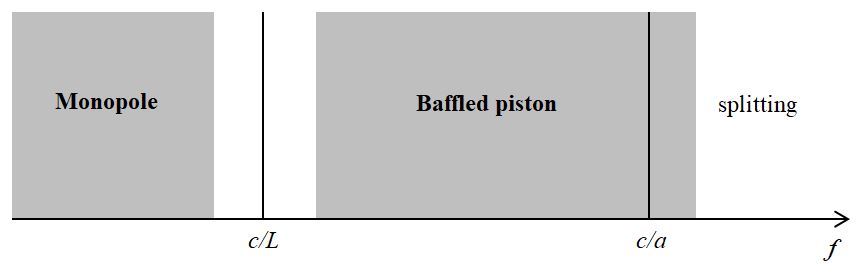
We have seen in this article the different models of sound sources that can explain the radiation of the membrane of a loudspeaker.
The dipole model showed that it was necessary to enclose the loudspeaker in a box to suppress the back wave and avoid the acoustic short circuit responsible for a significant power loss, mainly at low frequencies.
Le modèle simple de la sphère pulsante est une bonne approximation du comportement d’une enceinte aux basses fréquences.
For higher frequencies, the more complete baffled piston design should be preferred.
At very high frequencies, the membrane splits and no simple model can account for its exact behavior.
These different areas are summarized in the figure below:
We are now equipped to deal with the electrodynamic speaker in the next article!
Sources
Optique – José-Philippe Pérez
Le cours d’acoustique de ECAN Lyon
Rayonnement acoustique – UPMC – Institut Jean Le Rond d’Alembert
Haut-parleurs et enceintes acoustiques : Théorie et pratique – Francis BROUCHIER

