Category: Physics of sound

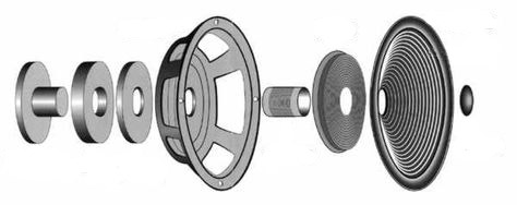
This article follows thestudy of the electroacoustic speaker. We will see here what happens to its properties and its radiation when it is integrated into a cabinet to make a loudspeaker.

• Resonance of a driver mounted in a cabinet
  • Pressure variations in the cabinet
  • Mechanical equation
  • Resonance frequency
• Acoustic radiation
  • Transfer function
  • Baffle step
  • Radiated power in both models
  • Baffle step transition
  • Sound level
• Diffraction from the edges
  • The problem
  • Case of a circular baffle
  • Off-axis observation
  • Rectangular baffle
• Conclusion

Resonance of a driver mounted in a cabinet

Pressure variations in the cabinet

As we have seen, the opposite phase emission from the rear side of the membrane creates harmful destructive interferences, especially in the low frequency range. The integration of the loudspeaker in a cabinet aims to avoid this acoustic short-circuit: the rear radiation is in fact suppressed.

Let V_0 the volume of the box, enclosing air at atmospheric pressure P_0. The volume of air contained in the sealed cabinet varies with the displacement of loudspeaker membrane of surface S when the elongation of the membrane is x, the air volume is V=V_0 + \Delta V with \Delta V = S \cdot x. The air undergoes a succession of compressions and expansions during the vibrations of the membrane.

If we assume, as usual, that these transformations are adiabatic, it follows from Laplace's law that:

\displaystyle{ \frac{ \text d}{\text d V} \left( P\cdot V^\gamma \right) = 0 \iff \frac{ \text{d}P}{\text{d}V} = - \frac{\gamma P}{V} }

Hence, if the volume \Delta V swept by the membrane remains small compared to the total volume of the chamber V_0the resulting overpressure can be written as :

\displaystyle{ p = - \frac{\gamma P_0}{V_0} \Delta V = - \frac{\gamma P_0}{V_0} S x }

Mechanical equation

Let's follow the application of Newton's second law to the loudspeaker seen previously, we obtained the mechanical equation of the speaker:

(m + 2m_\text{R}) \cdot \ddot{x} + (\alpha + 2R_\text{R}) \cdot \dot{x} + k \cdot x = Bl \cdot i

Two changes must be made in the configuration of the closed enclosure:

• On the one hand, since the back radiation has been removed, the factor 2 in front of the radiation resistance R_\text{R} disappears.
• One the other hand, the overpressure p of air enclosed in the cabinet adds a force F whose expression is, according to the result of the previous paragraph : F = p\cdot S = - \frac{\gamma P_0 S^2}{V_0} x
  This is a recall force F = - k_\text{a} \, x, with k_\text{a} = \frac{\gamma P_0 S^2}{V_0} the stiffness of the volume of air enclosed in the box.

Assuming that the surface area of the diaphragm is small compared to the surface area of the front panel of the housing, the mass of air displaced at the back of the diaphragm is approximately equal to that displaced at the front. The total mass of the moving assembly will therefore remains m+2m_R

The mechanical equation of the loudspeaker mounted in a cabinet is therefore :

\displaystyle{ \boxed{ (m + 2m_\text{R}) \cdot \ddot{x} + (\alpha + R_\text{R}) \cdot \dot{x} + \left( k + k_\text{a} \right) \cdot x = Bl \cdot i }}

The behavior of the loudspeaker mounted in a closed box can therefore be deduced from that of the loudspeaker mounted on an infinite plane baffle by the substitutions :

• 2R_\text R \rightarrow R_\text R
• k \rightarrow k_\text{b} = k + k_\text a with k_\text a = \frac{\gamma P_0 S^2}{V_0}

We will use the index b for all quantities related to the speaker mounted in a box.

Resonance frequency

Following the approach we used for the speaker mounted on a plane baffle, we end up with the equivalent electrical diagram of the speaker mounted in a box:

The motional resistance and inductance are unchanged, but the motional capacitance undergoes a change:

\displaystyle{\left\{ \begin{array}{ll} L_{\text{m,b}} = \frac{m +2m_\text{R}}{(Bl)^2}\\ R_{\text{m,b}} = \frac{(Bl)^2}{\alpha} \\ C_{\text{m,b}} = \frac{(Bl)^2}{k_\text b} \end{array}\right.}

It follows that the resonance of the motional circuit R,L,C in parallel will occur at the pulsation :

\displaystyle{\left( \frac{\text{d}\underline{Z}_\text{mot}}{\text{d}\omega}\right)_{\omega=\omega_b} = 0 \iff \omega_b = \frac{1}{\sqrt{L_{\text{m,b}} \cdot C_{\text{m,b}}}} = \sqrt{\frac{k_b}{m + 2m_\text{R}}}}

The numerator of the expression is larger than in the case of a flat baffle mounting, and the denominator is the same: the resonance frequency of the loudspeaker is therefore increased when it is installed in a cabinet.

The speaker mounted in a cabinet will therefore have a higher bass cut-off frequency.

The loss of emission in the bass will be all the more marked as the stiffness k_\text a of the air contained in the chamber will be important, this one increasing when the volume V_0 of the cabinet decreases. The crossover frequency of the speaker will be multiplied by \sqrt{2} when k_\text a = k. This threshold gives the order of magnitude of the minimum volume of the box to be used.

It is customary to introduce here the air volume equivalent to the suspension V_\text{as}, usually published in the loudspeaker manufacturer's data. The stiffness k of the loudspeaker would be obtained with a volume of air

\boxed{ \displaystyle{ V_\text{as} = \frac{\gamma P_0 S^2}{k} }}

To mount a loudspeaker in a closed cabinet without increasing the crossover frequency too much, you will need a cabinet volume at least a few times greater than V_\text{as}.

Example

Let's illustrate these words with a numerical example. Let's recall the manufacturer's data of the Monacor SP-165PA loudspeaker that we took as an example in the previous article: :

• Effective membrane area S = 137\times10^{-4}\,\text{m}^2
• Mass of the moving part (coil + membrane) m = 8,2\times10^{-3} \,\text{kg})
• Stiffness of the elastic suspension k = 4,0\times 10^{3} \,\text{N}\,\text{m}^{-1})
• Mechanical resistance of the suspension \alpha= 1,2 \,\text{kg}\,\text{s}^{-1}
• Coil's resistance R_e = 6.9\,\Omega
• Coil's inductance L_e= 0,50 \times10^{-3} \,\text{H}
• Force factor Bl = 7,1 \,\text{T}\,\text{m}

We have for this speaker \displaystyle{ V_\text{as} = 6,6 \,\text{L} }. If one chooses to mount it in a volume box V_0=40\,\text{L} \approx 6 V_\text{as}we will have : k_\text a = \frac{\gamma P_0 S^2}{V_0} = 6,7 \times 10^2 \,\text{N}\,\text{m}^{-1}

The total stiffness will be: k_\text b = k + k_\text a = 4,7 \times 10^3 \,\text{N}\,\text{m}^{-1}

And the resonance pulsation: \omega_\text b = \sqrt{\frac{k_b}{m + m_\text{R}}} = 654 \, \text{rad} \, \text{s}^{-1} = 1,08 \, \omega_0

The cutoff frequency will have increased by 8%, from 96 to 104 Hz.

Acoustic radiation

Transfer function

The equivalent acoustic diagram for the speaker mounted in a cabinet is :

• Excitatory pressure \underline{p}_g=\underline{P}_g \exp (j\omega t) with \underline{P}_g = \frac{(Bl)\cdot\underline{U}}{S\cdot R_e}, in units of Pascals.
• Acoustic flow \underline{q} = \underline{Q} \exp (j\omega t), in \text{m}^3/\text{s}
• Acoustic resistances, in units of \text{Pa}\cdot\text{s}/\text{m}^3:
  • R_{ae}=\frac{(Bl)^2}{S^2 R_e} (electrical losses in the coil)
  • R_{ab}=\frac{\alpha}{S^2} (frictional losses)
• Acoustic compliance, in units of \text{m}^3/\text{Pa} : C_{ab}=\frac{S^2}{k_b}.
• Acoustic mass, in units of \text{kg}/\text{m}^4 : M_{ab}=\frac{m + m_\text{R}}{S^2}
• Acoustic resistance of front radiation, R_{ar}=\frac{R_\text{R}}{S^2}

Let's call:

• \delta = \frac{\omega_b}{\omega_s} = 1,08 ;
• Q_{eb} =\frac{1}{\omega_b C_{ab}R_{ae}}  the electrical quality factor ;
• Q_{mb} =\frac{1}{\omega_b C_{ab}R_{ab}}  the mechanical quality factor ;
• Q_{tb}   the total quality factor such that \frac{1}{Q_{tb}} = \frac{1}{Q_{eb}} + \frac{1}{Q_{mb}} .

Let's take the example of the Monacor already studied, mounted in a 40 L box:

Mounting on a flat baffle	Mounting in a 40 L box
\omega_s = 606 \, \text{rad}\,\text{s}^{-1}	\omega_b = \delta \omega_s = 654 \, \text{rad}\,\text{s}^{-1}
Q_\text{es} = 1,1	Q_{eb}=1,0
Q_\text{ms} = 5,0	Q_\text{mb} = 4,6
Q_\text{ts} = 0,91	Q_\text{tb} = 0,83

The quality factors decrease when the loudspeaker is integrated into a cabinet, the smaller the volume of the cabinet.

The expression for the flow, obtained by following the approach outlined in the previous article, is then :

\displaystyle{ \underline{Q}_b = \frac{j\delta \nu}{( j \delta \nu)^2 +\frac{j \delta \nu}{Q_{tb}} + 1} \cdot \omega_b C_{ab} \underline{P}_g = \frac{j\delta \nu}{( j \delta \nu)^2 +\frac{j \delta \nu}{Q_{tb}} + 1} \cdot \frac{ \omega_s C_{as}}{\delta} \underline{P}_g }

where \nu = \frac{\omega}{\omega_s} is the reduced pulsation defined with respect to the resonance pulsation of the planar baffle speaker and where the second term has been rewritten according to the values of the planar baffle speaker.

Baffle step

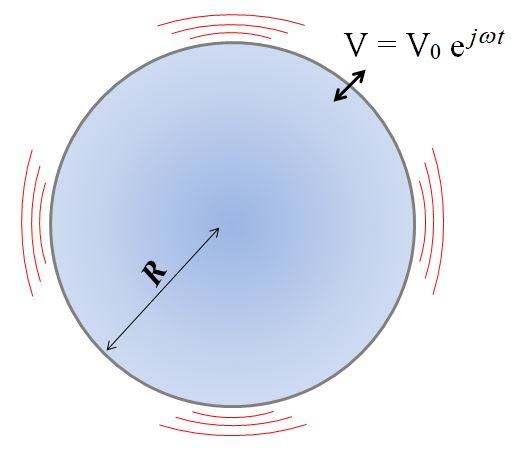
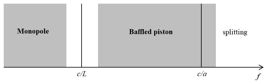
When we studied the acoustic monopoleWe have reported that it models the radiation of a closed enclosure at very low frequencies in a very satisfactory way. Indeed, the wavelength being greater than the dimensions L of the baffle (f < c / L), this one is invisible for the emitted sound waves. The radiation is then isotropic in all space.

Then we studied the model of the piston embedded on an infinite baffle, which accurately models the radiation from a speaker at higher frequencies (f > c / L): the wavelength being smaller than the baffle of the box, the sound waves see it as a large baffle. The radiation is then mainly in the front half space. As long as the wavelength is greater than the radius a of the loudspeaker, this radiation is also mostly non-directional.

In the transfer function obtained in the previous paragraph, it will therefore be necessary to use the monopole model for low frequencies and the baffled piston model for higher frequencies. The transition between these two models is called baffle step, or baffle step transition .

Radiated power in both models

The radiated power is obtained from the transfer function in the same way as we obtained it for the radiation of the speaker mounted on an infinite baffle. The difference between the monopole radiation (low frequency) and that of the baffled piston (high frequency) is the radiation resistance R_R, which is doubled for the baffled piston. We thus obtain for the baffled piston:

\displaystyle{ { \mathcal{P}_{ar,b,\text{HF}} = \frac{\rho_0}{4\pi c} \left( \frac{\omega_s^2 C_{as} \underline{P}_g}{\delta^2} \right) ^2 \left|\underline{H}_{P,b}\right|^2} \hspace{1cm} \text{avec} \hspace{1cm}\underline{H}_{P,b} = \frac{\delta^2\nu^2}{( j\delta\nu)^2 +\frac{j\delta\nu}{Q_{tb}} + 1} }

In the monopole case, we get twice as much:

\displaystyle{ { \mathcal{P}_{ar,b,\text{BF}} = \frac{\rho_0}{8\pi c} \left( \frac{\omega_s^2 C_{as} \underline{P}_g}{\delta^2} \right) ^2 \left|\underline{H}_{P,b}\right|^2}} = \frac{ \mathcal{P}_{ar,b,\text{HF}}}{2}

In the low frequencies, the maximum value of the radiated power is thus divided by 2\delta^4 compared to the same loudspeaker mounted in a flat baffle. In order to optimize the bass cutoff frequency and the sound level, it is therefore in the best interest of the speaker to place it in a cabinet with a sufficiently large volume so that \delta close to 1.

The efficiency \eta_b of the loudspeaker mounted in a closed cabinet is calculated in the high frequencies, where \left|\underline{H}_{P,b}\right| \approx 1 : we thus have \eta_b = \frac{\eta_0}{\delta^4}. In our example, we get 0,6\%.

The sensitivity L_{1,b} of the enclosure is reduced by 10\cdot \log{\delta^4}, i.e. a drop of 1,3\,\text{dB} for the considered enclosure: we obtain L_1 = 90,2\,\text{dB}.

Baffle step transition

At high frequencies, the sound waves are emitted in the front half of the cabinet. At a distance r from the speaker, the emitted power is diluted on a half-sphere of surface 2\pi r^2 and the sound intensity is:

\displaystyle{ I_\text{HF} = \frac{ \mathcal{P}_{ar,b,\text{HF}} }{2\pi r^2}}

At low frequencies, sound waves are emitted in all space, the surface on which the energy is diluted is therefore 4\pi r^2. Then we have :

\displaystyle{ I_\text{BF} = \frac{ \mathcal{P}_{ar,b,\text{BF}} }{4\pi r^2} = \frac{I_\text{HF}}{4}}

The transition linked to the baffle step is therefore accompanied by a decrease of 6\text{dB} in the bass.

On which frequencies does the baffle step spread?

The diffraction is quantified by the angle \theta of the wave spreading. For the obstacle of dimension L that is the cabinet of the speaker, we have :

\theta = \frac{\lambda}{L}

A wave emitted by the loudspeaker along the baffle will be significantly diffracted to the rear when \theta \approx \frac{\pi}{4}. This corresponds to \lambda_1 \approx 0,7L. The radiation will become isotropic in space when \theta \approx 2\pi, that is \lambda_2 \approx 6 L. The transition frequency is the one for which the attenuation is half of its maximum value, i.e. :

f_\text{step} = \sqrt{f_1 f_2} = \sqrt{\frac{c^2}{\lambda_1\lambda_2} } \approx \frac{1}{2} \frac{c}{L}
f_1 \approx 3 \, f_\text{step}, f_2 \approx \frac{f_\text{step}}{3}

Or

\lambda_\text{step} = \frac{c}{f_\text{step}} \approx 2L
\lambda_1 \approx \frac{\lambda_\text{step}}{3}, \lambda_2 \approx 3 \, \lambda_\text{step}

A good mathematical model of the transition can be constructed using a well-known approximation of the Heavyside step function :

H(f) \approx 6 \times \left( \left( 1 + \exp{ \left( -2 k \ln{\frac{f}{f_\text{step}}} \right) } \right)^{-1} -1 \right)

with k=2 allowing the spreading of the phenomenon over the interval \left[ \frac{f_\text{step}}{3} ; 3 \, f_\text{step} \right] :

Sound level

We can now calculate the sound intensity at high frequencies with the expression obtained above, deduce the sound level and take into account the transition to monopole radiation at low frequencies by adding the baffle step transition.

For our 40L loudspeaker, let's choose a depth of the cabinet of 25 cm and a circular baffle of 22,5 cm of radius, the loudspeaker being mounted in the center of it. I don't recommend such a geometry, but it allows to have only one dimension L=0,45 \,\text{m} to consider. We obtain, with a baffle phenomenon at 380 Hz ranging from 127 Hz to 1.14 kHz :

It should be noted, however, that in a real case of listening in a room, a significant fraction of the bass sound waves emitted towards the back of the speaker will be reflected by the walls, thus increasing the perceived level of the bass. The baffle phenomenon will therefore cause a decrease of 2 to 4 dB rather than 6 dB.

Note also that, when the box is rectangular, the transition will be smoothed out due to different transition frequencies for the different sizes of the obstacle seen by the wave :

For example, for the same box volume of 40L and the same depth of 25cm, a rectangular baffle of dimension 30 \times 50 \,\text{cm} will have a transition of baffle phenomenon that will extend from \lambda_1 \approx 0,7 \,L_{min}=21\,\text{cm} at \lambda_{max} \approx 6 \,L_{max}=3,0 \,\text{m}, that is:

f_{min}=114\,\text{Hz} \,\, ; \,\, f_{max}=1,63\,\text{kHz}, \,\,f_\text{step}=\sqrt{f_{min}f_{max}}=430\,\text{Hz}

Diffraction from the edges

The problem

In this section, we are interested in the "high-frequency" side of the baffle step: the sound waves are supposed to propagate in a half-space delimited by the baffle.

Let us consider a spherical wave. The Huygens-Fresnel principle states that each point of the medium perturbed by the wave becomes itself a secondary elementary source, the combination of the perturbations generated by these secondary sources constituting the new wave front:

When the wave propagating along the baffle reaches its periphery, it encounters a discontinuity since the volume available for its propagation changes: it passes from a half-sphere to a sphere. The pressure drops by a factor of 2 and the secondary sources no longer form a coherent whole with their predecessors, they must be considered as a new source. We speak of diffraction by the edge of the baffle.

Due to their phase shift, resulting from the delay induced by the propagation to the edge of the baffle, the direct wave and the diffracted wave interfere at the point of observation: the sound pressure will show peaks when the waves are in phase and troughs when they are in phase opposition.

Case of a circular baffle

In order to simplify and focus on the physical effects, we will first restrict ourselves to the unfavorable case of a circular baffle observed on axis.

We are interested here in high frequencies: let us thus change our loudspeaker of study for a tweeter Dayton DC28FT of radius a=14 \,\text{mm}, of resonance frequency f_s = 834 \,\text{Hz} and of total quality factor Q_\text{ts} = 0,50. This loudspeaker is mounted in a closed enclosure, in the center of a circular baffle of radius R= 22,5 \,\text{cm}. There is no modification of the resonance frequency for the tweeter: it is factory mounted in an airtight box (the box would serve, in a real case of two-way speaker, to remove the acoustic short circuit of the bass speaker).

Its theoretical response curve is then, taking into account the baffle step:

The distance covered by the wave when reaching the edge of the baffle is equal to the radius R of the baffle. The edge of the baffle thus behaves like a second source emitting at the same frequency as the loudspeaker but with a delay \tau = R/c, the time it takes to reach the edge of the baffle from its center.

The direct wave propagating in a half-space is at point M :

\displaystyle{ p_0 = \frac{j \omega \rho Q_0}{2\pi} \cdot \frac{\exp{j \left( \omega t - k r_0\right) }} {r_0} }

The diffracted wave emitted by an infinitesimal secondary source of length \text{d}\mathcal{l} = R\cdot \text{d}\varphi is written as follows:

\displaystyle{ \text{d}p_1 = D(0) \cdot \frac{j \omega \rho Q_0}{4\pi} \cdot \frac{ \exp{ \left[ j \left( \omega t - k \left(r_1+R\right) \right)\right]} } {r_1 + R} \cdot \frac{\text{d}\varphi}{2\pi} }

where D(0) is the directivity factor of the speaker along the baffle.

In far field, we have r_1 \approx r_0 and the difference in amplitude due to the additional distance traveled R is negligible. Therefore:

\displaystyle{ \text{d}p_1 = D(0) \cdot \frac{1}{2} \cdot p_0 \cdot \exp{\left( -j k R \right)}\frac{\text{d}\varphi}{2\pi} }

The integration along the circle is trivial, finally:

\displaystyle{ p_1 = D(0) \cdot \frac{1}{2} \cdot p_0 \cdot \exp{\left( -j k R \right)} }

The resulting pressure at the observation point is therefore :

\displaystyle{ p = p_0 + p_1 = p_0 \left( 1 + D(0) \cdot \frac{1}{2} \exp{ \left(- jkR \right) } \right) }

Direct and diffracted waves interfere at the observation point via the term in parentheses; the effective sound pressure is :

\displaystyle{ p_\text{eff} = \frac{ \left| p \right| }{\sqrt{2}} = p_{0,\text{eff}} \left( 1 + D(0) \cdot \frac{1}{2} \cos{ \left(kR\right) }\right) }

The interference will be constructive when the direct and diffracted waves are in phase at the observation point, i.e. when k R = m \cdot2\pi with m a positive integer, that is \lambda = R/m or f = m c /R. The waves will be in phase opposition, generating destructive interference, when k R = \left( m + \frac{1}{2} \right) \cdot2\pi, that is \lambda = R/\left( m + \frac{1}{2} \right) or f = \left( m + \frac{1}{2}\right) c /R.

The speaker becomes very directional at high frequencies (ka >= 4the phenomenon fades away:

The sound level variations are therefore of the order of 10 dB maximum (the pressure varies by a factor of 3 between 0.5 and 1.5, the sound intensity varies by a factor of 9 and 10 \times \log{9} = 9,5.

We can now compute the sound intensity I=\frac{p_\text{eff}^2}{\rho c} and the resulting sound level:

The first trough, corresponding to \lambda / 2 = R, is partially hidden by the baffle step (the wavelength is long, the radiation of the speaker is therefore almost on a sphere and there is little diffraction). The first bump at the end of the baffle-step transition corresponds to \lambda = R then the next trough at \lambda = \frac{2}{3}R, etc.

Let us observe an enlargement of the area of interest, in linear frequency scale:

The peaks are spaced at about 1500 Hz, the corresponding wavelength is \lambda = \frac{c}{f} = 22,8\,\text{cm} : we can thus measure the radius of the baffle.

Note here that the amplitude of the variations will be reduced by rounded edges.

Off-axis observation

We now place ourselves off-axis, in a direction defined by the angle \eta relative to the axis of symmetry of the baffle:

A little bit of geometry allows us to see that the additional path difference of the diffracted wave relative to the direct wave is \delta = R \sin{\eta}\cos{\varphi}, the corresponding phase shift is \phi_0 = k\delta.

The direct wave has therefore the expression :

\displaystyle{ p_0 = D\left(\frac{\pi}{2}-\eta\right) \cdot \frac{j \omega \rho Q_0}{2\pi} \cdot \frac{\exp{j \left( \omega t - k r_0\right) }} {r_0} }

And we will have at the observation point, for an infinitesimal secondary source \text{d}p_1 :

\displaystyle{ \text{d}p_1 = D(0) \cdot \frac{1}{2} \cdot p_0 \cdot \exp{\left( -j k (R - \delta) \right)}\frac{\text{d}\varphi}{2\pi} }

The wave diffracted by the edge of the baffle is thus :

\displaystyle{ p_1 = D(0) \cdot \frac{1}{2} \cdot p_0 \cdot \exp{\left( -j k R\right)} \cdot \int_0^{2\pi} \exp{\left( j k R\sin{\eta}\cos{\varphi}) \right)} \frac{\text{d}\varphi}{2\pi} }

The integral in the last term is : J_0\left(k R \sin(\eta)\right), Bessel function of order 0 :

\displaystyle{ p_1 = D(0) \cdot \frac{1}{2} \cdot p_0 \cdot \exp{\left( -j k R\right)} \cdot J_0\left(k R \sin(\eta)\right) }

Summing the direct wave p_0 (affected by the directivity factor D(\frac{\pi}{2}-\eta) ) and the diffracted wave p_1, then calculating the corresponding sound intensity and deducing the sound level in the same way as before, we obtain the following curves:

It is not surprising to see that the diffraction by the edges is smaller off-axis: indeed, the various secondary sources around the baffle are no longer all in phase. This calculation shows that when we try to correct the peaks and troughs on-axis by digital filtering, we generate peaks and troughs off-axis.

Rectangular baffle

Let's take a look at the more concrete case of the rectangular baffle, observed on axis. Its geometry is summarized in the following figure:

We have kept the dimensions of the box used in the calculation of the baffle phenomenon: L_1=50\,\text{cm}, L_2=30\,\text{cm}. The tweeter is located at the coordinates x_t = y_t = 20\,\text{cm}.

The expression of the direct wave is identical to that obtained in the case of the circular baffle, and an infinitesimal source located at the coordinate \varphi will generate at the observation point, with the same simplifications as before:

\displaystyle{ \text{d}p_1 = D(0) \cdot \frac{1}{2} \cdot p_0 \cdot \exp{\left( -j k b(\varphi) \right)}\frac{\text{d}\varphi}{2\pi} }

The integration is done numerically, by pieces for each of the edges of the baffle. For example, for the upper edge, we have :

\displaystyle{ p_{1,\text{top}} = D(0) \cdot \frac{1}{2} \cdot p_0 \cdot \int_{\arctan{\frac{L_1-y_t}{L_2-x_t}}}^{\frac{\pi}{2}+\arctan{\frac{x_t}{L_1-y_t}}} {\exp{\left( -j k \frac{L_1-y_t}{\sin{\varphi}} \right)}\frac{\text{d}\varphi}{2\pi} } }

The interference term has the shape given below.

We deduce the sound level of the loudspeaker mounted in the cabinet as above:

As expected, the effects of diffraction by the edges of the baffle are much less pronounced than with a circular baffle (the secondary sources are never all in phase with the direct wave). Here, as with the circular baffle, the measurement of the frequency differences of the different peaks allows us to deduce the distance between the loudspeaker and the edges of the baffle. For example, the two most visible peaks on the graph are 3400 Hz apart, which corresponds to a wavelength of 10 cm, the distance between the loudspeaker and the top of the cabinet.

The directivity study is also performed by numerical integration, adding the additional step difference as in the case of the circular baffle \delta = b(\varphi)\cdot\sin{\eta}\cdot\cos{\varphi} :

Conclusion

We have seen in this article the consequences on the acoustic radiation of the sealing of a loudspeaker in a box: increase of the resonance frequency, baffle phenomenon and diffraction by the edges of the baffle.

A possible way to counter the increase of the resonance frequency and thus of the low cutoff of the loudspeaker is to integrate a vent in the cabinet to realize a bass-reflex speaker. The next article will be dedicated to this system.

Sources

Francis BROUCHIER – Haut-parleurs et enceintes acoustiques : Théorie et pratique

Jean Fourcade – Utilitaires Scilab pour le calcul et l’optimisation d’enceintes bass-reflex

Loudspeaker Cabinet Diffraction (Tore Skogberg)

Diffraction from baffle edges

After covering the basics of acoustics and the acoustic radiation, this article will discuss the problem of producing sound waves with an electroacoustic speaker. We will build on what we learned there and use the principle of electromagnetic induction as well as some mechanics to understand how an electrodynamic loudspeaker works. The model we will build will allow us to identify the important physical quantities and to discuss the order of magnitude of their values.

• Technical data of a speaker
  • Description
  • Set of parameters
• Mechanical equation
  • Lorentz force
  • Laplace force exerted on a conductor
  • Special case of a speaker's coil
  • Fundamental principle of dynamics
• Electrical equation
  • Induced electromotive force
  • Mesh equation
• Impedance
  • Sinusoidal steady state solutions
  • Equivalent electrical circuit
• Acoustic radiation
  • Equivalent acoustical circuit
  • Acoustic flow
  • Radiated power
  • Efficiency
  • Sound level, sensitivity
  • Displacement of the diaphragm
• Maximal values
  • Voltage and electrical power
  • Sound level
• High frequencies
• Conclusion

Technical data of a speaker

Description

Set of parameters

• Effective membrane area S = 137\times10^{-4}\,\text{m}^2
• Mass of the moving part (coil + membrane) m = 8,2\times10^{-3} \,\text{kg})
• Stiffness of the elastic suspension k = 4,0\times 10^{3} \,\text{N}\,\text{m}^{-1}) (its inverse, compliance, is frequently found C = 1/k in units of \text{m}\,\text{N}^{-1})
• Mechanical resistance of the suspension \alpha= 1,2 \,\text{kg}\,\text{s}^{-1} (coefficient of the velocity in the expression of the drag)
• Coil's resistance R_e = 6.9\,\Omega (the index e refers to electrical quantities)
• Coil's inductance L_e= 0,50 \times10^{-3} \,\text{H}
• Force factor Bl = 7,1 \,\text{T}\,\text{m} (product of the magnetic field strength by the length of the coiled wire)

To which we add the limit value of the diaphragm excursion for which the response is linear: x_\text{max} = 3,75 \times10^{-3} \,\text{m}

Mechanical equation

Lorentz force

Adding up these two forces, we get the Lorentz force qui s’exerce sur une particule chargée plongée dans un champ électromagnétique :

\vec{F}=q \cdot (\,\vec{E} + \vec{v} \land \vec{B})\,

Laplace force exerted on a conductor

Consider a wire-shaped electrical circuit, through which a current Iflows, in motion in an electromagnetic field (\, \vec{E},\,\vec{B} )\, at velocity \vec{V}.

All charged particles in the conductor (metal ions and free electrons) are subject to the Lorentz force.

For the metal ions, of positive charge, e standing for the elementary charge:

\vec{F}_{ion}=e \cdot (\,\vec{E} + \vec{V} \land \vec{B})\,

For free electrons, of opposite charge moving at speed \vec{u} in the circuit:

\vec{F}_{elec}=-e \cdot (\,\vec{E} + (\,\vec{V} + \vec{u})\,\land \vec{B})\,

There are as many metal ions as free electrons. All the contributions cancel out except the one due to the electrons' own speed in the circuit. The force exerted globally on the circuit, called Laplace force, is thus the sum of all \vec{f}=-e \vec{u}\land \vec{B} exerted upon each of the free electrons.

Special case of a speaker's coil

To simplify the following, let's place ourselves in the geometry that interests us for the study of the loudspeaker. The conductor is a coil of wire of total length l immersed in a radial magnetic field of intensity B :

According to the right hand rule, for a current flowing clockwise (and thus electrons flowing counterclockwise) all the forces to be summed are therefore collinear to the central axis of the device, directed along the increasing x . This is the convention chosen on the loudspeakers: the terminal tinted red or marked "+" corresponds to the direction of connection for which a positive current sets the moving equipment in motion towards the exterior. We still have to add up the contributions \vec{f}=-e\cdot u\cdot B \cdot \vec{e}_x for each free electrons (\vec{e}_x est le vecteur unitaire portant l’axe x).

How many free electrons are there in this coil? The current being the flow of charges, there are n=I/e electrons that cross a section of the circuit in one second. The last ones to cross it are those which were located at a distance \delta = u \times 1\,\text{s} one second before. If l is the length of the wire, there are therefore \frac{l}{\delta} times more : there is a total of N = n \cdot \frac{l}{\delta}=\frac{I \cdot l}{u\cdot e} free electrons. The Laplace force exerted on the coil is finally :

\vec{F}_L=N \cdot \vec{f}=\frac{I \cdot l}{u\cdot e} \cdot (\,-e)\,\cdot u\cdot B \cdot \vec{e}_x=I \cdot Bl \cdot \vec{e}_x

If the coil is traversed by a current of constant intensity i, the Laplace force exerted on it will therefore also be constant. But if we impose a variable current i in the coil, we see that the Laplace force will also be variable. It will push the coil sometimes to the right (when the current is positive) and sometimes to the left (when it is negative). The effect will be to make the coil vibrate around its equilibrium position.

The mechanical vibratory energy can then be transmitted in part to the air, as we have detailed in the previous article.

Finally, note that the Laplace force is proportional to the force factor Bl we can find on the speaker's specs.

Fundamental principle of dynamics

Let us apply the fundamental principle of dynamics to the system {coil + membrane} of mass m dans le référentiel de l’aimant : m \cdot \vec{a} = \Sigma\, \vec{F}_\text{ext}.

The forces exerted along the x axis are:

• the return force -k\cdot x due to the elastic fixation, which brings the system back to its equilibrium position;
• a dissipative force of fluid friction proportional to the speed of the system -\alpha \cdot v_x = -\alpha \cdot \dot{x} ;
• the Laplace force Bl \cdot i exerted on the coil ;
• the pressure forces -p_\text{avant} S and p_\text{arrière} S due to the pressure of the air on the faces of the membrane. These forces characterize the acoustic radiation of the loudspeaker.

We saw that the pressure forces were written: Z_\text{R} \cdot \dot{x}, with Z_\text{R} = R_\text{R} + j \omega m_\text{R} the radiation impedance. The expressions of the radiation resistance R_\text{R} and the radiation mass m_\text{R} are, for a piston embedded in an infinite plane, in the low frequency approximation :

\displaystyle{ R_\text{R} \approx \rho c S \sigma = \frac{\rho_0 S^2 }{2\pi c}\omega^2 \hspace{1cm}\text{et} \hspace{1cm} m_\text{R} \approx \frac{8\rho}{3}\left(\frac{S}{\pi}\right)^{3/2} }

For the Monacor speaker taken as an example, we get:

\displaystyle{ R_\text{R} \approx 1,0\times10^{-7}\omega^2 \;\text{kg}\,\text{s}^{-1}\hspace{1cm}\text{et} \hspace{1cm} m_\text{R} \approx 0,9 \,\text{g} }

The radiation resistance is therefore negligible compared to the mechanical resistance up to \omega \approx 10^3 \,\text{rad}\,\text{s}^{-1}. The expression used is in any case only valid at low frequencies. The radiation mass implies a small correction of a few percent.

In contrast to the solid piston model, the loudspeaker diaphragm is in contact with the air on both sides of the baffle: radiation mass and radiation resistance must be taken into account for the front radiation and for the back radiation.

We thus obtain the differential equation for the position of the coil (mechanical equation of the speaker:

(m + 2m_\text{R}) \cdot \ddot{x} = -k \cdot x - (\alpha + 2R_\text{R})\cdot \dot{x} + Bl \cdot i

Electrical equation

Induced electromotive force

When a circuit is mobile in a magnetic field, the magnetic force exerted on the free electrons will set them in motion. An induced current therefore appears spontaneously in the circuit. We call electromotive force u_\text{ind} the potential difference explaining the appearance of this electric current. We will establish in this paragraph the expression of the e.m.f. induced in the coil of a loudspeaker moving in the magnetic field of the magnet.

In the reference frame of the magnet, there is in the gap a radial magnetic field \vec{B} . When the coil is moving at the speed \vec{V}, the free electrons undergo a Lorentz force \vec{F}=-e \cdot \vec{V} \land \vec{B}. According to the right hand rule, this force will tend to set the electrons in motion in the trigonometric direction, and thus generate a positive current in the coil. By calling \vec{u} the unit vector directed at each point of the coil in the direction of a positive intensity : \vec{F}= e \cdot V \cdot B \cdot \vec{u}.

Let's place ourselves now in the reference frame of the coil. We have just seen that electrons initially at rest will start moving clockwise. They are thus subjected to the effect of an electric field \vec{E}' which is written, by definition :

\displaystyle{ \vec{E}' = \frac{\vec{F}}{q} = \frac{e \cdot V \cdot B \cdot \vec{u}}{-e}= V \cdot B \cdot \vec{u} }

The induced electromotive force is equal to the electric field circulation between the two ends of the coil;

u_\text{ind}= \int_0^l \vec{E}' \cdot \text d \vec{l} =- V \cdot Bl

Mesh equation

The mesh equation yields:

u(t)\, + u_\text{ind}(t)\, = u_R + u_L \, \iff \, R \cdot i + L \cdot \frac{\text{d}i}{\text{dt}} = u(t)\, - Bl \cdot \dot{x}

This equation is called electrical equation of the speaker. It is therefore, unsurprisingly, the equation of a steady state R,L circuit. But the voltage forcing the circuit contains two terms: the imposed voltage and the e.m.f. due to the speed of the coil.

Impedance

Sinusoidal steady state solutions

We have seen that the radiation resistance is small compared to the mechanical friction coefficient: R_\text{R} \ll \alpha. We will thus neglect the term containing R_\text{R} in this section which only deals with the electrical behavior of the loudspeaker.

A speaker is therefore governed by two equations:

\left\{ \begin{array}{ll} (m + 2m_\text{R})\cdot \ddot{x} + \alpha \cdot \dot{x} + k \cdot x = Bl \cdot i \\ R \cdot i + L \cdot \frac{\text{d}i}{\text{dt}} = u(\,t)\, - Bl\cdot \dot{x} \end{array}\right.

These equations are coupled, since the mechanical equation contains the electrical variable i and the electrical equation contains the mechanical variable x. The coupling coefficients are respectively Bl and - Bl : they are opposed to one another.

Let us look for particular solutions of these equations by imposing a sinusoidal regime. A more complex sound will be described by a set of frequencies, and thus by a sum of sinusoids, as explained here. Let's impose in the mechanical equation a sinusoidal intensity \underline{i}=\underline{I} \cdot \exp{(\,j \omega t)\,}. We use here the complex notation.

Let us now inject into the equation a sinusoidal solution for xi.e. a solution written as \underline{x}=\underline{X} \cdot \exp{(\,j \omega t)\,}. We get:

\left[(m + 2m_\text{R}) (j \omega)^2 + j \omega \alpha + k \right] \cdot \underline{X} = Bl \cdot \underline{I}

Operating in the same way for the electrical equation :

\underline{U} - Bl \cdot \underline{\dot{X}}= \left( R + j \omega L \right) \underline{I}

Eliminate \underline{X} of the second equation using the first :

\displaystyle{\underline{\dot{X}} = \frac{ j \omega \cdot Bl}{(m + 2m_\text{R}) (j\omega)^2 +j \omega \alpha + k} \cdot \underline{I}}

\displaystyle{\underline{U} = \left( R + j \omega L + \frac{j \cdot \omega \cdot (Bl)^2}{(m + 2m_\text{R}) (j\omega) ^2 +j \omega \alpha + k}\right)\underline{I}}

Where theimpedance of the speaker \underline{Z} = \underline{U} / \underline{I} appears:

\displaystyle{\underline{Z} = R + j \omega L + \frac{j \omega \cdot (Bl)^2}{(m + 2m_\text{R}) (j\omega)^2 -j \omega \alpha + k} }

The term R + j \omega L is the classical electrical impedance of a coil, the second term is due to the movement of the coil in the magnetic field of the magnet and is called motional impedance: :

\displaystyle{\underline{Z}_{\text{mot}} = \frac{j \omega \cdot l^2 \cdot B^2}{(m + 2m_\text{R}) \omega ^2 -j \omega \alpha - k} }

Equivalent electrical circuit

Note now that the motional impedance can be written :

\displaystyle{\underline{Z}_{\text{mot}} = \frac{1}{\frac{j \omega (m + 2m_\text{R})}{(Bl)^2} + \frac{\alpha}{(Bl)^2} +\frac{k}{j \omega (Bl)^2}} }

That is:

\displaystyle{\frac{1}{\underline{Z}_{\text{mot}}} = \frac{1}{j \omega L_\text{mot}}+ \frac{1}{R_\text{mot}} + \frac{1}{\frac{1}{j\omega C_\text{mot}} } }

with

\displaystyle{\left\{ \begin{array}{ll} L_{\text{mot}} = \frac{m + 2m_\text{R}}{(Bl)^2}\\ R_{\text{mot}} = \frac{(Bl)^2}{\alpha} \\ C_{\text{mot}} = \frac{(Bl)^2}{k} \end{array}\right.}

We thus recognize the association in parallel of a capacitor of capacity C_{\text{mot}}a resistor of resistance R_{\text{mot}} and a coil of inductance L_{\text{mot}}.

For the speaker used as an example, we obtain :

• C_{\text{mot}} = 198 \,\text{µF}
• R_\text{mot} = 42,0 \,\Omega
• L_\text{mot}= 12,6 \,\text{mH}

Let's take a moment to understand the physical origin of these three effects. The moving mass allows the storage of energy (due to inertia) like a coil stores magnetic energy when charged particles moves accross it. Friction forces dissipate energy as does a resistance by Joule effect. Finally, the stiffness of the spring allows, by the return force, the storage of elastic energy, as a capacitor stores electrical energy by adding up charges on both plates.

The equivalent electrical diagram of a loudspeaker is finally :

The resonance of the motional circuit R_{\text{mot}}, \, L_{\text{mot}} , \, C_{\text{mot}} in parallel occurs at the pulse

\displaystyle{\left( \frac{\text{d}\underline{Z}_\text{mot}}{\text{d}\omega}\right)_{\omega=\omega_0} = 0 \iff \omega_0 = \frac{1}{\sqrt{L_{\text{mot}} \cdot C_{\text{mot}}}} = \sqrt{\frac{k}{m + 2m_\text{R}}}}.

In our example, \omega_0 = 606\,\text{rad}\,\text{s}^{-1} that is f_0 = 96\,\text{Hz}. The peak of the impedance modulus is |\underline{Z}|_\text{max}=R_e+R_\text{mot}=49\,\Omega.

Two important facts to note here:

• The impedance peak at the resonance frequency f_0 = \frac{\omega_0}{2\pi} implies that the speaker cannot generate sound at a lower frequency. This frequency is therefore the low limit of the bandwidth. In fact, although it is marketed by displaying its power, an amplifier is indeed an amplifier of voltage. But the power is \mathcal{P} = \frac{U^2}{|\underline{Z}|}: it collapses when the frequency gets close to the impedance peak's.
• At low frequencies, the electrical impedance of the speaker is almost resistive: \underline{Z}_{e} = R_e + j\omega L_e \approx R_e. But when the pulsation approaches the value \omega = R_e/L_e (in our example, close to 14 000 \,\text{rad}\,\text{s}^{-1}), the inductive effects start to appear and the impedance rises.
• Between those two values, the modulus of the impedance passes through a minimum Zwhich is the impedance displayed by the manufacturer.

Only the acoustic performance of a speaker is, in fineof interest. The electrical study has however of interest that the measurement of the impedance curve, simpler to realize with precision than an acoustic measurement, allows to determine certain acoustic characteristics of the loudspeaker (motional resistance, resonance pulsation).

Acoustic radiation

Equivalent acoustical circuit

Let's start again from the mechanical equation and the electrical equation and eliminate the current from the mechanical equation. We obtain without difficulty :

\displaystyle{\frac{Bl\cdot\underline{U}}{R_e+j\omega L_e} = \left[ j\omega (m+2m_\text{R}) + (\alpha + 2R_\text{R}) + \frac{k}{j\omega} + \frac{(Bl)^2}{R_e + j\omega L_e} \right] \cdot \underline{\dot{X}} }

It is an equality between terms of the dimension of a force, i.e. energy per unit length. By dividing by the surface of the speaker S, we therefore obtain an equality between pressures (the Pascal is an energy per unit of volume):

\displaystyle{ \frac{(Bl)\cdot\underline{U}}{S(R_e+j\omega L_e)} = \left[ \frac{ j\omega (m+2m_\text{R})}{S^2} + \frac{\alpha + 2R_\text{R}}{S^2} + \frac{k}{j\omega S^2} + \frac{(Bl)^2}{S^2(R_e + j\omega L_e)} \right] \cdot \underline{Q}}

where \underline{q} = S \cdot \dot{\underline{x}} = \underline{Q} \exp{(j \omega t)} is the acoustic flow of the speaker.

At low frequencies (\omega \ll R_e/L_e), the left-hand term is independent of the frequency:

\displaystyle{ \frac{(Bl)\cdot\underline{U}}{S\cdot R_e} = \left[ j\omega \frac{m + 2m_\text{R}}{S^2} + \frac{\alpha + 2R_\text{R}}{S^2} + \frac{1}{j\omega} \frac{k}{S^2} + \frac{(Bl)^2}{S^2\cdot R_e} \right] \cdot \underline{Q}}

We then obtain an "electrical" equation describing a series association of four resistors, a capacitor and a coil:

\displaystyle{ \underline{P}_g = \left(R_{ae} + R_{as} + \frac{1}{j\omega \, C_{as}} + j\omega M_{as}+R_{ar,1}+R_{ar,2} \right) \cdot \underline{Q}}

With:

• The equivalent of the voltage is the excitation pressure \underline{p}_g=\underline{P}_g \exp (j\omega t) with \underline{P}_g = \frac{(Bl)\cdot\underline{U}}{S\cdot R_e}, in units of Pascals.
• The corresponding current is the acoustic flow (or volume velocity) \underline{q} = \underline{Q} \exp (j\omega t), in \text{m}^3/\text{s}
• The acoustic resistances are, in \text{Pa}\cdot\text{s}/\text{m}^3:
  • R_{ae}=\frac{(Bl)^2}{S^2 R_e} (electrical losses in the coil)
  • R_{as}=\frac{\alpha}{S^2} (frictional losses)
• The acoustic compliance (equivalent of a capacity) is, in \text{m}^3/\text{Pa} : C_{as}=\frac{S^2}{k}. The compliance, widely used in acoustics, is the opposite of the stiffness.
• The acoustic mass (equivalent of an inductance) is, in \text{kg}/\text{m}^4 : M_{as}=\frac{m + 2m_\text{R}}{S^2}
• The front and back radiation acoustic resistances R_{ar,1}=\frac{R_\text{R}}{S^2} and R_{ar,2}= R_{ar,1}

The index s following the 'acoustic' index a correspond to the speaker (speaker) alone. We will change it for a b (box) when it is mounted in a case and the corresponding quantities are changed.

We can now solve the physical problem by analogy with an electrical circuit. The equivalent circuit is as follows:

Acoustic flow

Here too, given the low efficiency of the speakers, we can neglect the radiation resistances in the calculation of the speaker output. The transfer function of the loudspeaker is then written :

\displaystyle{  \underline{Q} = \frac{1}{R_{ae} + R_{as} + \frac{1}{j\omega \, C_{as}} + j\omega M_{as}}\cdot \underline{P}_g }

\displaystyle{ \iff \underline{Q} = \frac{1}{( j\omega)^2 C_{as} M_{as} + j \omega C_{as}R_{ae} + j \omega C_{as}R_{as} + 1} \cdot j \omega C_{as} \underline{P}_g }

It is the transfer function of an oscillator damped by the resistive terms, which therefore behaves like a bandpass filter. Its resonance pulsation is : \omega_s^2 = 1/(C_{as}M_{as}) = k/(m + 2m_\text{R}) = \omega_0^2. The resonance of the acoustic flow takes place at the frequency corresponding to the electrical impedance peak.

Let's call:

• \nu = \omega / \omega_s  the reduced pulsation ;
• Q_{es} =\frac{1}{\omega_s C_{as}R_{ae}}  the electrical quality factor (for the Moncaor Q_{es} = 1,11) ;
• Q_{ms} =\frac{1}{\omega_s C_{as}R_{as}}  the mechanical quality factor (for the Monacor Q_{ms}= 5,0).

The expression of the acoustic flow becomes:

\displaystyle{ \underline{Q} = \frac{j\nu}{( j\nu)^2 + j\nu \left(\frac{1}{Q_{es}}+ \frac{1}{Q_{ms}}\right) + 1} \cdot \omega_s C_{as} \underline{P}_g }

Let's finally call Q_{ts}   the total quality factor such that \frac{1}{Q_{ts}} = \frac{1}{Q_{es}} + \frac{1}{Q_{ms}} (in our example, we have Q_{ts} = 0,91 ):

\displaystyle{\boxed{ \underline{Q} = \frac{j\nu}{( j\nu)^2 +\frac{j\nu}{Q_{ts}} + 1} \cdot \omega_s C_{as} \underline{P}_g }}

Radiated power

We know that:

\displaystyle{ \mathcal{P}_{ar} = R_\text{R} V_\text{eff}^2 = \frac{R_\text{R}}{S^2} Q_\text{eff}^2 = \frac{R_\text{R}}{2 S^2} |Q|^2}

Furthermore R_\text{R} = \rho_0 c S \sigma. We get:

\displaystyle{ \mathcal{P}_{ar} = \frac{\rho_0 c \sigma}{2 S} |Q|^2}

We are here in low frequency approximation with respect to the characteristics of the speaker (\omega \ll \frac{R_e}{L_e}). The low frequencies with respect to the acoustic characteristics are defined by ka \ll 1 \iff \omega \ll \frac{c}{a} (a being the radius of the membrane).

In our example, we have a = \sqrt{S/\pi} = 0,066 \, \text{m} : \omega \ll \frac{c}{a} \approx 5 000 \, \text{rad}\cdot \text s ^{-1} \approx 800 \, \text{Hz}

These two approximations are therefore of the same order of magnitude. In their respect ( f < 300 \, \text{Hz}), the radiation factor of the baffled speaker is, as already used above, \sigma \approx \frac{a^2 k^2}{2} = \frac{S}{2\pi c^2}\omega^2. We get:

\displaystyle{ \mathcal{P}_{ar} = \frac{\rho_0 }{4\pi c}\omega^2|Q|^2 }

The response curve of the speaker at low frequencies is then, by injecting the expression of the acoustic flow's amplitude :

\displaystyle{ \boxed{ \mathcal{P}_{ar} = \frac{\rho_0 \left( \omega_s^2 C_{as} \underline{P}_g \right) ^2}{4\pi c} \left|\underline{H}_P\right|^2} \hspace{1cm} \text{avec} \hspace{1cm} \boxed{\underline{H}_P = \frac{\nu^2}{( j\nu)^2 +\frac{j\nu}{Q_{ts}} + 1} }}

On the form a+jb, the transfer function is written:

\displaystyle{ \underline{H}_P = \frac{ \displaystyle{\frac{\nu^3}{Q_{ts}}}+j \nu^2 (1-\nu^2)} {\nu^4 + \nu^2 \left(-2 + \displaystyle{\frac{1}{Q_{ts}^2}} \right) + 1} }

Its squared modulus is therefore:

\displaystyle{ |\underline{H}_P|^2 = \frac{\nu^4} {\nu^4 + \nu^2 \left(-2 + \displaystyle{\frac{1}{Q_{ts}^2}} \right) + 1} }

At low frequencies \nu \rightarrow 0, an expansion at first non-zero order yields |\underline{H}_P|^2 \approx \nu^4. The asymptotic behavior of the sound level is thus a straight line with a slope of 12 dB/octave (the power is indeed multiplied by 2^4=16  when the frequency doubles).

The square of the modulus of the transfer function is as follows:

We see on the previous expression that there will be a resonance (red and purple curves above) only if -2 + \frac{1}{Q_{ts}^2} < 0 \iff Q_{ts} > 1/\sqrt{2}. A good speaker will ensure a smooth transition to the bass and will therefore not have a pronounced power peak: it will have a maximum quality factor Q_{ts} \leq \frac{1}{\sqrt{2}}.

The cut-off at 3\,\text{dB} occurs when |\underline{H}_P|^2 = \frac{1}{2}, that is:

\nu_3^2 = \left( \frac{1}{2Q_{ts}^2}-1\right) + \sqrt{1+\left( \frac{1}{2Q_{ts}^2}-1\right)^2}

With numerical values:

In order for it to provide maximum power until cut-off (as opposed to the blue and orange curves which collapse early), a good speaker will therefore have a total quality factor close to Q_{ts} \approx 1/\sqrt{2} \approx 0,7 (green curve).

The speaker we're studying, with Q_{ts} \approx 0,9is close to the red curve. From the point of view of the -3 dB cutoff in the bass, it is rather good. From the point of view of a smooth transition to the bass, it is not an excellent choice.

Efficiency

The efficiency of the speaker is:

\displaystyle{ \eta = \frac{\mathcal{P}_{ar}}{\mathcal{P}_e} }

where \mathcal{P}_e = \frac{U_\text{eff}^2}{|\underline{Z}|} is the electrical power consumed by the loudspeaker. As these quantities depend on the frequency, the efficiency will be evaluated at the minimum of the impedance module, for which |\underline{Z}| \approx R_e and |\underline{H}_P| = 1. We thus have:

\displaystyle{ \eta_0 = \frac{\rho_0}{4\pi c} \frac{ \left(\omega_s^2 C_{as} \underline{P}_g \right) ^2}{U_\text{eff}^2/R_e} }

Developing the expression of the excitation pressure, we get:

\displaystyle{ \eta_0 = \frac{\rho_0}{4\pi c} \frac{ \left(\omega_s^2 C_{as} \frac{(Bl)\sqrt{2}U_\text{eff}}{S\cdot R_e} \right) ^2}{U_\text{eff}^2/R_e} = \frac{\rho_0}{2\pi R_e c} \left( \frac{\omega_s^2 C_{as}(Bl)}{S} \right) ^2 }

That, in turns, becomes as a function of the speaker's parameters only:

\displaystyle{ \boxed{ \eta_0 = \frac{\rho_0}{2\pi R_e c} \left( \frac{S(Bl)}{m + 2m_\text{R}} \right) ^2 }}

The numerical value for our example is: \eta_0 = 0,8\%.

The efficiency of a loudspeaker is generally less than 1%, which justifies in another way to have neglected in the previous calculations the radiation resistance.

Sound level, sensitivity

In the far field, the radiation from the diaphragm is isotropic. The sound intensity at a distance r is thus obtained by dividing the acoustic power by the surface of the half-sphere on which the energy is diluted:

I = \displaystyle{ \frac{\mathcal{P}_{ar}}{2\pi r^2} = \frac{\rho_0}{8\pi^2 c}\left(\frac{\omega_s^2 C_{as} \underline{P}_g}{r} \right)^2 \left| \underline{H}_P \right|^2 }

The sound level is, by definition:

L=10\, \log \frac{I}{I_0}

The sensitivity L_1 of a speaker is the sound level obtained at a distance of r_0 = 1 \,\text{m} from the loudspeaker when supplied with an RMS voltage U_\text{eff}= 2,83V (which, for an impedance of 8 \Omegacorresponds to an average electrical power \mathcal{P}_e = U_\text{eff}^2/Z=1\,\text{W}). The sensitivity is evaluated in the frequency range where the speaker is most effective (|\underline{H}_P| = 1).

Using this definition, we can write:

\displaystyle{ L_1=10\, \log \frac{\eta_0 U_\text{eff}^2 / (2\pi R_e)}{I_0}=10\, \log \frac{ U_\text{eff}^2}{2\pi I_0} + 10\, \log \frac{\eta_0}{R_e} = 121,1 + 10\, \log \frac{\eta_0}{R_e} }

This relationship yields, when applied to the woofer : L_1 = 91,5\,\text{dB}.

Displacement of the diaphragm

The excursion of the membrane \underline{x} = \underline{X} \exp (j \omega t) = \frac{\underline{V}}{j\omega} \exp (j\omega t) is obtained from the expression of the volume velocity:

\displaystyle{ \underline{X} = \frac{\underline{V}}{j \nu \omega_s} = \frac{\underline{Q}}{j \nu \omega_s S} = \frac{1}{j\nu \omega_s S} \frac{j\nu}{( j\nu)^2 +\frac{j\nu}{Q_{ts}} + 1} \cdot \omega_s C_{as} \underline{P}_g }

That is:

\displaystyle{ \underline{X} = \underline{H}_X \cdot \frac{C_{as} \underline{P}_g}{S} }

with \displaystyle{ \underline{H}_X = \frac{1}{( j\nu)^2 +\frac{j\nu}{Q_{ts}} + 1} }

whose modulus is \displaystyle{ |\underline{H}_X| = \frac{1}{\sqrt{\nu^4 +\nu^2\left(-2+\frac{1}{Q_{ts}^2}\right) + 1} } }

As for the power, there will be no resonance for a good loudspeaker with a total quality factor equal or very close to 1/\sqrt{2}. In this case, the maximum displacement is at \nu=0 :

Maximal values

Voltage and electrical power

The effective displacement of the loudspeaker depends on the voltage imposed by the amplifier (appearing in the expression of the excitation pressure \underline{P}_g). The maximum permissible voltage is therefore the voltage at which the loudspeaker reaches its maximum linear elongation x_\text{max}.

But at which frequency should we do this calculation?

• On the one hand, the displacement is maximal at low frequencies
• On the other hand, we have seen that the power collapses when attacking the impedance peak of the speaker.

We can then estimate the maximum voltage required by doing the calculation at half the peak of the motional impedance: we select \omega_p such that |\underline{Z_\text{mot}}|(\omega_p)=\frac{|\underline{Z}|_\text{mot,max}}{2}.

The expression of the motional impedance can be put in the form :

\displaystyle{ |Z_\text{mot,p}|^2=\left( \frac{R_\text{mot}}{2} \right)^2 = \frac{\omega_p^2 (Bl)^4}{(m + 2m_\text{R})^2\omega_p^4 + (\alpha^2 - 2 (m+2m_\text{R}) k) \omega_p^2 + k^2} }

The solution of the second degree equation in \omega_p^2 leads in our example to : f_p = 108 \,\text{Hz}.

The displacement of the membrane to be taken into account for this calculation is therefore :

\displaystyle{ |\underline{X}| = |\underline{H}_X(\omega_p)| \cdot \frac{C_{as} P_g} {S} }

Let us inject the expression of the excitation pressure and impose |\underline{X}|=x_\text{max}:

\displaystyle{ x_\text{max} = |\underline{H}_X(\omega_p)| \cdot \frac{C_{as} (Bl)\cdot U_\text{max}}{S^2\cdot R_e} = |\underline{H}_X(\omega_p)| \cdot \frac{(Bl)\cdot U_\text{max}}{k\cdot R_e} }

We get:

\displaystyle{ U_\text{max} = \frac{1}{ |\underline{H}_X(\omega_p)| }\cdot \frac{k R_e x_\text{max}} {Bl} }

For the woofer we find U_\text{max}=22\,\text{V}. The maximum power required from the amplifier is then \mathcal{P}_{e,\text{max}} = \frac{U_\text{max}^2}{R_e}= 68\,\text W. The latter is calculated not at the impedance peak but at its minimum value \approx R_e. The speaker's datasheet indicates 50 \,\text W_\text{RMS} and 100 \,\text W at peak, but it corresponds only to electrical and not acoustic criteria.

Maximum sound level

We can now recalculate the sound level with the maximum peak voltage we just obtained:

\displaystyle{ L_\text{max}=10\, \log \frac{ U_\text{max}^2/2}{2\pi I_0} + 10\, \log \frac{\eta_0}{R_e} }

For the Monacor Woofer, we get: L_\text{max}=112\,\text{dB}. As we will see in the next article, and as many other results obtained here, this value will be modified when placed in a box.

High frequencies

The radiated power was calculated in the low frequency approximation. We have indeed used an expansion of the radiation factor for ka \ll 1, which corresponds to a limit frequency for our example f \ll 830 \,\text{Hz}. Moreover, the radiation resistance at high frequencies is no longer negligible compared to the mechanical resistance. Finally, the low-frequency approximation results in the quasi-isotropic emission of the loudspeaker, and we have therefore neglected its directivity.

All the previous calculations are therefore valid, as we have already said, only for frequencies lower than a few hundred Hertz. But the loudspeaker that we study is announced to be able to emit from 93 Hz (its resonance frequency) to 5500 Hz.

Let's compare the model we have developed (in red) with the measured response curve of the speaker:

If the model explained in this article is very efficient to determine the properties of a loudspeaker at low frequencies, it is insufficient to characterize its high cutoff frequency and the sometimes pronounced "accidents" appearing on the response curve. For example, the SP-165PA shows a sudden drop in sound level around 1 kHz, then oscillations that appear around 5 kHz.

What can be predicted about the radiation of the speaker beyond the low frequency approximation? This will be the subject of a future article to provide some answers.

Conclusion

In this article, we have presented a model of the electro-dynamic speaker embedded in an infinite baffle, allowing to understand the phenomena at work behind the response curve and to calculate precisely this curve at low frequencies. The low frequency domain is particularly useful to predict the low cutoff frequency of the loudspeaker, the required electrical power, and the expected maximum sound level.

In the next article, we will see how these quantities are modified when the loudspeaker is embedded in a cabinet to make a loudspeaker.

Sources

José-Philippe Pérez – Mécanique (DUNOD)

Modélisation électrique et acoustique du haut-parleur : impédance électrique et bande passante acoustique

Francis BROUCHIER – Haut-parleurs et enceintes acoustiques : Théorie et pratique

Jean Fourcade – Utilitaires Scilab pour le calcul et l’optimisation d’enceintes bass-reflex

After having introduced the bases de l’acoustique, we will focus in this article on the radiation of acoustic energy. We will see how to use the already established acoustics formulas to calculate the sound intensity generated by a vibrating solid. We will focus on the three cases that we will need to understand, later, the acoustic radiation of a loudspeaker: the pulsing sphere, the acoustic dipole, and the encased piston.

• Pulsing sphere model
  • Description
  • Acoustic pressure and velocity
  • The acoustic monopole
  • Sound intensity and level
  • Radiation's impedance
    • Formula
    • Radiation's mass and resistance
  • Radiation factor
  • Radiated acoustic power
• Acoustic dipole
  • Description
  • Acoustic pressure
  • Acoustic velocity
  • Sound intensity
• The baffled circular piston
  • Description
  • Huygens-Fresnel principle
  • Acoustic pressure
  • Sound intensity
  • Radiation's impedance
  • Radiated acoustic power
  • Limits of the model
• Conclusion

Pulsing sphere model

Description

The source considered here is a solid sphere of radius R whose surface oscillates at the uniform speed \underline{V} = V_0 \exp{(j \omega t)}. The amplitude of the oscillations is assumed to be small compared to the radius R. The air pressure is thus disturbed and a sine sound wave is emitted.

The symmetry of the problem indicates that the acoustic quantities depend only on time and distance r to the source. Hence the sound waves emitted by the pulsing sphere are spherical.

Acoustic pressure and velocity

The corresponding formulas in the case of spherical waves are :

\displaystyle{ \underline{p} = \frac{\underline{A}}{r} \exp{ \left[ j(\omega t - kr) \right] } }

\displaystyle{ \underline{u}_r = \left( 1 - \frac{j}{kr}\right) \frac{\underline{p}}{\rho_0 c} }

At the interface between the sphere and the air, the velocity of the air is equal to that of the surface of the sphere. The constant \underline{A} can therefore be determined. Let's inject the expression of the pressure into that of the velocity for r = R, et égalisons avec l’expression de la vitesse de la surface de la sphère :

\displaystyle{ \underline{u}_r (R) = \left( 1 - \frac{j}{kR}\right) \frac{\underline{A}}{\rho_0 c R} \exp{ \left[ j(\omega t - kR)\right] } = V_0 \exp{(j\omega t)} }

We get:

\displaystyle{ \underline{A} = \rho_0 c R V_0 \frac{ \exp{(jkR)} }{1-\frac{j}{kR}} = j \omega \rho_0 R^2 V_0 \frac{ \exp{(jkR)} }{1 + jkR} }

Note that this "constant" depends on the vibration frequency of the source!

The acoustic pressure is then:

\displaystyle{ \underline{p} = j \omega \rho_0 R^2 V_0 \frac{\exp{(jkR)} }{1 + jkR} \frac{\exp{ \left[ j(\omega t - kr) \right] }}{r} }

Now we define the acoustic flow Q of the source as the volume displaced by its vibrations per unit time: Q = Q_0 \exp{(j\omega t)} = 4 \pi R^2 V . The expression of \underline{p} becomes:

\displaystyle{ \underline{p} = \frac{ j \omega \rho_0 Q_0}{4\pi} \cdot \frac{\exp{(jkR)}}{1 + jkR} \cdot \frac{\exp{ \left[ j(\omega t - kr) \right] }}{r} }

As for the acoustic speed \underline{u}:

\displaystyle{ \underline{u}_r = \left( 1 - \frac{j}{kr}\right) \frac{ j \omega Q_0}{4\pi c} \cdot \frac{\exp{(jkR)}}{1 + jkR} \cdot \frac{\exp{ \left[ j(\omega t - kr) \right] }}{r} = \left( 1 + jkr \right) \frac{ Q_0}{4\pi} \cdot \frac{\exp{(jkR)}}{1 + jkR} \cdot \frac{\exp{ \left[ j(\omega t - kr) \right] }}{r^2}}

The acoustic monopole

It is difficult to design a loudspeaker whose membrane is a sphere, and one could doubt the importance of the previous calculation ... However, the model of the pulsating sphere will be of great use to us for the following two reasons:

• When the wavelengths are large compared to the dimensions of the speaker, it is experimentally verified that the acoustic radiation produced is very close to that of a pulsating sphere. The pulsating sphere is therefore a good model for the bass of an enclosure, even if only a part of the surface of the sphere vibrates. For the dimensions of the radios we use, about 50 cm, we can describe correctly by this model wavelengths greater than 1.5m, which corresponds roughly to frequencies below 200 Hz.
• Finally, by virtue of the Huygens-Fresnel principle, a complex vibrating source (the membrane of a loudspeaker) can be described below by considering it as a sum of spherical elementary sources.

Note that, in these two applications, the dimensions R of the source are small (relatively for the first, infinitesimal for the second). We can therefore simplify the expressions by making the radius of the sphere tend towards zero to obtain the expressions of the acoustic monopole :

\displaystyle{ \boxed{ \underline{p} = \frac{ j \omega \rho_0 Q_0}{4\pi} \cdot \frac{\exp{ \left[ j(\omega t - kr) \right] }}{r} }} \displaystyle{\underline{u}_r = \left( 1 + jkr \right) \frac{ Q_0}{4\pi} \cdot \frac{\exp{ \left[ j(\omega t - kr) \right] }}{r^2}}

Sound intensity and level

We have already shown that, for a spherical wave : \displaystyle{ I = \frac{p_\text{eff}^2}{\rho_0 c}}

Thus, the sound intensity of the wave produced by an acoustic monopole is :

\displaystyle{\boxed{ I = \frac{\rho_0 }{2c} \left( \frac{ \omega Q_0}{4\pi r} \right)^2 } }

As we have already mentioned when discussing geometric attenuation, the sound intensity decreases as the square of the distance to the source. The emitted energy is diluted over an area that increases as the square of the distance.

The sound level generated by the monopole results from this:

L(r) = 10 \log{ \frac{I(r)}{I_0} } = 10 \log{ \left[ \frac{\rho_0 }{2 I_0 c} \left( \frac{ \omega Q_0}{4\pi r} \right)^2 \right]} = 10 \log{ \left( \frac{\rho_0 }{32 \pi^2 I_0 c}\right) + 20 \log \left( \frac{ \omega Q_0}{r} \right)}

where, after the last equality, the only variable quantities are grouped in the last term.

Finally, the acoustic power \mathcal{P}_\text{s} émise par la source est calculable en sommant l’intensité sonore sur une sphére centrée sur la source de rayon r\prime :

\mathcal{P}_\text{ac} = 4\pi r\prime^2 I(r\prime) \iff \displaystyle{\boxed{ \mathcal{P}_\text{ac} = \frac{\rho_0 }{8\pi c} \left( \omega Q_0\right)^2 }}

Radiation's impedance

Formula

Let's go back to the pulsating sphere of radius R . By vibrating, it generates pressure variations in the air in its vicinity. These pressure variations generate, in turn, a force on the surface of the source. There is thus a phenomenon of coupling between the source and the environment it disturbs.

This force is naturally written : \underline{f} = - \underline{p}(R) \cdot S

where S = 4 \pi R^2  is the surface of the pulsating sphere, and where the negative sign comes from the fact that the force exerted by the air is directed towards decreasing r .

We showed that:

\displaystyle{ \underline{p}(R) = j \omega \rho_0 R^2 V_0 \frac{\exp{(jkR)} }{1 + jkR} \frac{\exp{ \left[ j(\omega t - kR) \right] }}{R} = \rho_0 R j \omega V_0 \exp{ (j\omega t)} \frac{1 }{1 + jkR}}

We have seen that the model of the pulsating sphere was valid only at low frequencies, that is kR \ll 1At first order it yields: \left( 1 + jkR \right)^{-1} \approx 1 - jkR :

\displaystyle{ \underline{p}(R) \approx \rho_0 R (1 - jkR) j \omega V_0 \exp{ (j\omega t)} = \rho_0 (1-jkR) j \omega \underline{V} = \left[ \frac{\rho R \omega^2}{c} + j \omega \rho_0 R \right] \underline{V} }

The force exerted by the air on the vibrating structure is thus:

\underline{f} = \left[- \frac{\rho R S \omega^2}{c} - j \omega \rho_0 R S \right] \underline{V}

We define theradiation impedance Z_{\text{ray}} as the ratio of the force \underline{f}\prime = -\underline{f} exerted by the vibrating surface on the air and the acoustic velocity \underline{u}(R) = \underline{V}(R) generated in the process:

\displaystyle{ Z_{\text{R}} = \frac{-\underline{f}}{\underline{u}} = \frac{\rho R S \omega^2}{c} + j \omega \rho_0 R S}

This quantity expresses the resistance of the air to vibrate under the action of the force.

Radiation's mass and resistance

Finally, we note that j \omega V_0 \exp{ (j\omega t)} corresponds to the acceleration \underline{a} of a point on the vibrating surface, so that the force can be written :

\displaystyle{ \underline{f} \approx -\rho_0 R S \underline{a} - \frac{\rho_0 R^2 \omega^2 S}{c} \underline{V} }

The coefficient \rho_0 R S of the acceleration is homogeneous to a mass that we will call radiation mass m_\text{R}. The second term is a fluid friction force of the type -R_\text{R} \underline{V}. R_\text{R} = \frac{\rho_0 R^2 \omega^2 S}{c} is the radiation resistance.

Thus, when we look for the equation of motion of the mobile part of a loudspeaker, Newton's second law will be written :

m \underline{a} = \Sigma \left(\text{autres forces}\right) + \underline{f}

\iff (m + m_\text{R}) \underline{a} = \Sigma \left(\text{autres forces}\right) - R_\text{R} \underline{V}

The radiation mass is interpreted as a mass of air moving along with the vibrating source. The radiation resistance is the friction coefficient translating the conversion of mechanical energy into acoustic energy: it explains the acoustic radiation of the structure.

With these notations, the radiation impedance is written :

\displaystyle{ \boxed{ Z_{\text{R}} = R_\text{R} + j \omega \, m_\text{R} }}

where

\displaystyle{R_\text{R} = \frac{\rho_0 S^2\omega^2 }{4\pi c} } \hspace{2cm}m_\text{R}= \rho_0 \frac{S^{3/2}}{2\sqrt{\pi}}

If the radiation mass of the pulsating sphere is kind enough to be a constant it is not the same for the radiation resistance which varies as the square of the pulsation. We can see from its expression that the conversion of mechanical energy of vibration of the source into acoustic energy will be very poor at low frequencies. Let's see this in detail.

Radiation factor

The radiation factor \sigma quantifies the efficiency of the conversion of mechanical energy of vibration into acoustic energy. It is defined by the relationship :

\displaystyle{ \boxed{ \sigma = \frac{\mathcal P_\text{ac}}{\rho_0 c S V_\text{eff}^2} }}

where the denominator corresponds to the acoustic power of the plane wave generated by an infinite plane vibrating at the same speed, measured on a surface equal to that of the source. Now, for the pulsating sphere, we have seen above that :

\displaystyle{ \mathcal{P}_\text{ac} =\frac{\rho_0 \omega^2 S^2 V_0^2}{8\pi c} }

Hence, the radiation factor of a pulsating sphere is :

\displaystyle{ \sigma = \frac{S \omega^2}{4\pi c^2} = R^2 k^2 }

The efficiency of the power transfer therefore varies as the square of the pulsation: it will be low in the bass, as has already been pointed out.

Note that the acoustic resistance can be written as a function of the radiation factor:

R_\text{R} = \rho_0 c S \sigma

An important fact should be noted here. Only one characteristic of the loudspeaker plays a role in the acoustic resistance and the radiation factor: its diameter (and therefore its surface). In terms of the efficiency of the transfer of mechanical energy from vibration to acoustic energy, the diameter of the loudspeaker is therefore the only factor that can be influenced.

To compensate for low transfer efficiency with a small loudspeaker, some manufacturers propose to increase the speed at which the membrane vibrates. For the same frequency of vibration, this consists in increasing the excursion of the loudspeaker membrane. But it is important to see that, in the formula giving the acoustic power, the surface is squared and therefore the diameter is to the power four: to obtain the same power with a loudspeaker of half the diameter, it would be necessary to increase the maximum excursion by a factor of four. If we look at the characteristics of "large excursion" loudspeakers, we realize that they are far from being able to compete with large loudspeakers in terms of bass reproduction.

Radiated acoustic power

We can now find the expression of the emitted power from the previous results. The fluid friction force -R_\text{R}\underline{V} described by the radiation resistance is responsible for the emission of acoustic waves.

The sound power is obtained by taking the scalar product of the force exerted by the source on the air with the speed of the air at the interface, its average is therefore :

\displaystyle{ \mathcal{P}_\text{ac} = \frac{1}{T} \, \int_0^T \Re(R_\text{R}\underline{V})\, \Re(\underline{V} )\text{d}t = R_\text{R}\frac{1}{T} \, \int_0^T \Re(\underline{V}\,\underline{V}^*) \text{d}t = R_\text{R} \frac{V_0^2}{2} }

That is:

\boxed{\mathcal{P}_\text{ac} = R_\text{R}V_\text{eff}^2 }

By sloting in the expression of the radiation resistance, we find the expression already calculated above:

\displaystyle{ \mathcal{P}_\text{ac} = \frac{\rho_0 R^2 \omega^2 S}{c}\frac{V_0^2}{2} = \frac{\rho_0 }{8\pi c} \left( \omega Q_0\right)^2 }

Acoustic dipole

Description

We get an acoustic dipole by placing at a short distance L \ll \lambda from each other two monopoles vibrating in phase opposition. We see here the interest of the modeling in this blog: when the membrane of a loudspeaker moves to the right, it generates an overpressure on the right and a depression on the left. A loudspeaker not mounted in a box behaves like a dipole.

The beautiful and simple spherical symmetry of the monopole is thus replaced by a cylindrical symmetry: the physical quantities will depend here, in addition to the coordinate r, of the coordinate \theta.

The two sources in phase opposition will generate interference. In particular, we can already see that, if the observer is placed at \theta = \frac{\pi}{2}, she will receive at the same time the opposite contributions of the two monopoles: the sound intensity will be zero.

Before going into details, let's see the dramatic consequences in terms of bass for the speakers. In order for the sound pressure to be maximal, let's place the observer on the axis y. For large wavelengths, the path difference between the two waves will be weak: the acoustic waves generated by the two monopoles will cancel almost entirely. The example below shows the result of this superposition for a wave of frequency f = 50 \,\text{Hz} and a distance L = 5 \, \text{cm}. The dotted curves indicate the pressure that would be observed with each monopole emitting alone, the green curve is the result of the superposition of the acoustic waves.

The sound pressure is divided by 20 between the monopole and the dipole in this example: the sound level produced by the dipole is therefore 20 \,\log 20 = 26 \text{dB} below that produced by a monopole of the same acoustic flow!

Acoustic pressure

Let's call Q_+ = Q_0 \exp{(j \omega t)} and Q_- = -Q_0 \exp{(j \omega t)} the acoustic flows of the two sources, which are opposite since they vibrate in phase opposition. The acoustic pressure obtained is of course the sum of the acoustic pressures coming from each of the monopoles:

\displaystyle{ \underline{p} = \underline{p}_+ + \underline{p}_- = \frac{ j \omega \rho_0 Q_+}{4\pi} \cdot \frac{\exp{ \left[-j kr_+ \right] }}{r_+} + \frac{ j \omega \rho_0 Q_-}{4\pi} \cdot \frac{\exp{ \left[ - j kr_- \right] }}{r_-} }

\displaystyle{ \iff \underline{p} = \frac{ j \omega \rho_0 Q_0}{4\pi} \cdot \left( \frac{\exp{ \left[- jkr_+ \right] }}{r_+} - \frac{\exp{ \left[ -jkr_- \right] }}{r_-} \right) \exp{(j \omega t)} }

We have r_+ and r_- close to r, therefore let's perform a Taylor expansion of the term in parentheses:

\frac{\exp (- jkr_+ ) }{r_+} \approx \frac{\exp (- jkr) }{r} + (r_+ - r) \frac{ \partial}{ \partial r} \left( \frac{\exp{(-jkr_+)}}{r_+}\right)_{r_+=r}

\iff \frac{\exp (- jkr_+ ) }{r_+} \approx \frac{\exp (- jkr) }{r} + (r_+ - r) (-\frac{1}{r}-jk) \frac{\exp{(-jkr)}}{r}

The same is done for the term containing the r_-, and we get:

\frac{\exp{ \left[- jkr_+ \right] }}{r_+} - \frac{\exp{ \left[ -jkr_- \right] }}{r_-} \approx (r_+ - r_-) (-\frac{1}{r^2}-\frac{jk}{r}) \exp (-jkr)

Let us now express r_+ -r_- using the diagram below and the good old Pythagorean theorem.

With (x,\,y) the Cartesian coodinates of the point Md’observation :

r_+^2 - r_-^2 = \left( x^2 + \left( y + \frac{L}{2}\right)^2\right) - \left( x^2 + \left( y - \frac{L}{2}\right)^2\right) = 2Ly = 2L r \cos \theta

Furthermore: r_+^2 - r_-^2 = (r_+ - r_-)(r_+ + r_-) \approx 2r(r_+ - r_-) d’où r_+ - r_- \approx L \cos \theta.

It comes then for the sound pressure :

\displaystyle{ \underline{p} = -\frac{ j \omega \rho_0 Q_0}{4\pi} \cdot L \cos \theta \left(\frac{1}{r^2}+\frac{jk}{r}\right) \exp (-jkr) \exp{(j \omega t)} }

That is:

\displaystyle{\boxed{ \underline{p} = \frac{ k^2 \rho_0 c L Q_0}{4\pi r} \, \cos \theta \, \left(1 + \frac{1}{jkr}\right) \exp [j(\omega t - kr)] }}

Unlike the radiation of the monopole, two terms appear here: one in 1/r^2 dominant in the near field (kr \gg 1), and one in 1/r dominant in the far field (kr \ll 1). The limit defining the far field depends of course on the frequency. But, for a typical listening distance of 3m, at 40 Hz :

kr = \frac{\omega}{c}r = \frac{2 \pi f}{c}r = \frac{2 \pi \times 40}{343}\times 3 = 2,19 > 1

The contribution of the near field will thus be weak for the low frequencies and totally negligible for the high frequencies: we are more interested in the far field for which

\displaystyle{ \underline{p}_\text{CL} = \frac{ k^2 \rho_0 c L Q_0}{4\pi r} \, \cos \theta \, \exp [j(\omega t - kr)] }

Acoustic velocity

We start as usual with the linearized Euler equation:

\displaystyle{\rho_0 j \omega\cdot \vec{\underline{u}} = - \vec{\nabla}\underline{p} }

with, in cylindrical coordinates, \vec{\nabla} = \frac{\partial}{\partial r} \vec{e}_r + \frac{1}{r}\frac{\partial}{\partial \theta} \vec{e}_\theta.

The radial coordinate is:

\displaystyle{ \underline{u}_r = -\frac{1}{j \omega \rho_0} \frac{\partial}{\partial r}\underline{p} }

\displaystyle{ \iff \underline{u}_r = \frac{k^2 Q_0 L}{4\pi r} \cos \theta \left( 1 + \frac{2}{jkr} - \frac{2}{(kr)^2} \right) \exp \left[j(\omega t - kr)\right] }

The orthoradial \theta coordinate is:

\displaystyle{ \underline{u}_\theta = -\frac{1}{j \omega r \rho_0} \frac{\partial}{\partial \theta}\underline{p} }

\displaystyle{ \iff \underline{u}_\theta = \frac{j k Q_0 L}{4\pi r^2} \sin \theta \left( 1 + \frac{1}{ jkr} \right) \exp \left[j(\omega t - kr)\right] } .

Sound intensity

Only the radial coordinate of the acoustic velocity is to be taken into account in the calculation, since the sound intensity corresponds to the power crossing a unit surface orthogonal to the direction of propagation of the wave. All calculations done, we obtain :

\displaystyle{ I = \frac{1}{2} \Re (\underline{p}\,\underline{u}_r^*) = \frac{\rho_0}{2c^3} \left( \frac{\omega^2 L Q_0}{4\pi r} \right)^2 \cos^2 \theta }

The sound level is deduced as usual:

L = 10 \, \log\left(\frac{I}{I_0}\right)

The radiation diagram of an acoustic dipole is shown below:

Acoustic power

It is obtained by integration of the sound intensity on a sphere centered on the origin, the surface element in spherical coordinates being : \text{d}S = \sin(\theta) r^2 \text{d}\theta \text{d}\phi :

\mathcal{P}_ \text{ac} = \int_0^{2\pi} \int_0^{\pi} I(r) \sin(\theta) r^2 \text{d}\theta \text{d}\phi

\iff \mathcal{P}_ \text{ac} = \frac{\rho_0c}{16 \pi} \left(k^2LQ_0 \right)^2 \int_0^{\pi} \cos^2 (\theta) \sin(\theta) \text{d}\theta

\iff \boxed{ \mathcal{P}_ \text{ac} = \frac{\rho_0 c \omega^4}{24 \pi c^3} \left(LQ_0 \right)^2 }

It depends, like the acoustic intensity, on the power 4 of the pulse, while the expression of the acoustic power for the monopole varied as \omega^2.

Comparing the two expressions, at identical acoustic flows leads to :

\displaystyle{ \frac{\mathcal{P}_\text{monopôle}}{\mathcal{P}_\text{dipôle}} = \frac{3}{(kL)^2}}

At low frequencies, this ratio is large: the dipole is much less efficient than the monopole to transfer its energy to the air. This result was already clearly visible on the radiation diagram.

This is due, as we have already said, to the destructive interference between the two sound waves. For an unmounted loudspeaker, which therefore behaves like a dipole, we speak of acoustic short circuit to describe this phenomenon of significant reduction of the power in the low frequencies: we can see the need to insert the speaker in a cabinet to suppress the rear wave. We will come back to this in an article on enclosed speakers.

The baffled circular piston

Description

We will establish here a model of the radiation of a loudspeaker membrane. In order to get rid of the back wave and the associated acoustic short circuit, the membrane will be considered embedded in an infinite (y,\, z) plane. Loudspeaker manufacturers will say that the speaker is baffled.

The membrane itself will be modeled as a circular piston of radius a and surface S=\pi a^2 and will as such be considered as flat and non-deformable. In this way, all the points of the membrane will have the same speed \vec{\underline{V}}(t) = V_0 \exp(j\omega t) and will therefore vibrate in phase.

Finally, we will limit ourselves to the calculation in far field: we will suppose kr \gg 1.

The situation being symmetrical by rotation around the (Oy)axis, it will be enough to calculate the acoustic quantities measured by observers M located in the (y, \,z)plane, and whose polar coordinates are M(r, \,\theta).

The model is summarized in the following diagram:

We will discuss the limitations of this modeling at the end of the section.

Huygens-Fresnel principle

We have here to calculate the acoustic quantities due to an extended source. The approach to tackle such a problem is the same as in optics when studying diffraction. The Huygens-Fresnel principle states that an extended source of surface S can be decomposed into spherical elementary sources of elementary surfaces \text{d}S. Acoustic quantities measured in M will be the sum of the contributions of these elementary sources.

We already have an elementary spherical source: it is obviously the acoustic monopole. However, a subtlety is introduced here. The monopoles emit on the supposedly perfectly rigid surface of the piston: the wave emitted towards the half-space y<0 is therefore reflected towards the front of the membrane. Thus, the acoustic pressure and velocity measured at the front of the membrane will be twice as important, while they will be null at the back.

The formula for sound pressure established at the beginning of the article becomes :

\displaystyle{ \underline{p} = \frac{ j \omega \rho_0 V_0\text{d}S}{2\pi} \cdot \frac{\exp{ \left[ j(\omega t - kr) \right] }}{r} }

Acoustic pressure

We thus have to integrate at observation point M the set of contributions of the elementary sources identified by their polar coordinates (\mathcal{l}, \, \psi) in the plane (x, \, z) :

\displaystyle{ \underline{p} = \frac{ j \omega \rho_0 V_0}{2\pi} \exp ( j\omega t) \int_0^{2\pi} \int_0^a \frac{\exp (- j k u)}{u} l\text{d}l \text{d}\psi }

In the far field approximation, M is at infinity, \vec{u} and \vec{r} are thus almost collinear. The figure below represents the plane containing the origin, M and \text{d}S , it allows us to see that u \approx r - l \cos \delta.

In addition, the relationships of spherical trigonometry let us write: \cos \delta = \cos \theta \cos \psi. The formula for pressure becomes:

\displaystyle{ \underline{p} = \frac{ j \omega \rho_0 V_0}{2\pi} \frac{\exp \left[ j(\omega t- kr)\right] }{r} \int_0^{2\pi} \int_0^a \exp ( j k l \cos \theta \cos \psi) l\text{d}l \text{d}\psi }

\iff \displaystyle{ \underline{p} = \frac{ j \omega \rho_0 V_0}{2\pi} \frac{\exp \left[ j(\omega t- kr)\right] }{r} \int_0^a l \left( \int_0^{2\pi} \exp ( j k l \cos \theta \cos \psi) \text{d}\psi \right) \text{d}l }

We just stumble across Bessel functions J_n regularly encountered in physics in problems with cylindrical symmetry, and whose results are known:

\left\{ \begin{array}{ll} J_0(X) = \frac{1}{2\pi} \int_0^{2\pi} \exp (j X \cos \psi) \text{d}\psi \\ J_1(X) = \frac{1}{X} \int_0^X u \, J_0(u) \text{d}u \end{array} \right.

The double integral becomes:

2\pi \int_0^a l J_0 \left(kl\cos\theta\right) \text{d}l

Then, by labeling u = kl\cos\theta :

\frac{2\pi}{k^2\cos^2\theta} \int_0^{ka\cos\theta} u \, J_0 (u)\, \text{d}u = \frac{2\pi a}{k\cos\theta}J_1 (ka\cos\theta) = S\cdot \frac{2J_1(ka\cos\theta)}{ka\cos\theta}

The acoustic pressure at point M is thus written:

\displaystyle{ \underline{p} = \frac{ j \omega \rho_0 Q_0}{2\pi} \frac{\exp \left[ j(\omega t- kr)\right]}{r} D(\theta) }

with \displaystyle{ D(\theta) = \frac{2 J_1(ka \cos\theta)}{ka \cos \theta} } the directivity factor.

We find here the expression of the sound pressure for a monopole emitting in a half-space with a directivity factor in tow, depending on \theta. In contrast to the dipole, the directivity here depends on the frequency of the emitted wave. The shape of the term D(\theta) is given in the following figure:

The speaker remains undirected at low ka, then becomes directional and secondary lobes appear at high frequencies.

Sound intensity

The sound pressure is the product of the sound pressure of a spherical wave by a real number. Therefore, we can use :

\displaystyle{\boxed{ I = \frac{p_\text{eff}^2}{\rho_0 c} = \frac{ \rho}{2c} \left( \frac{\omega Q_0}{2\pi r} \right)^2 D(\theta)^2}}

At low frequencies, the radiation is isotropic in the half-space and D(\theta) \approx 1. We thus have for identical flows:

I \approx 4 I_\text{monopôle}

A factor of 2 comes from an emission on a half space instead of the whole space, another one is explained by a double radiation resistance (see below). Let us note now that there will be a difference of 6dB in the sound level between a monopole emission and a baffled piston emission, all other things being equal.

The radiation diagram has the following appearance:

The pressure is divided by \sqrt{2} at u = 1,6 : the sound intensity is then divided by two and the sound level has dropped by 3 dB. Let's define the half aperture of the beam by the angle \eta = \frac{\pi}{2} - \theta_{-3\text{dB}} :

• Below ka = 1,6, \theta_{-3\text{dB}} doesn't exist and /eta = \frac{\pi}{2} the loudspeaker has a quasi-isotropic emission in the front half-space.
• Beyond that, we have \eta = \frac{\pi}{2} - \arccos \frac{1,6}{ka}.
• It remains roughly undirected until ka=3,9.
• It becomes highly directed beyond.

Radiation's impedance

A long calculation leads to the following result:

Z_\text{R} = \rho c S \left[ \sigma + j x_\text{R} \right]

with the radiation factor \sigma = 1 - \frac{J_1 (2ka)}{ka} and x_\text{R} = \frac{S_1 (2ka)}{ka}

where J_1 is Bessel function of order 1 and S_1 is Struve's. The radiation factor is therefore low for ka \ll 1 : the transfer of mechanical energy from the membrane into acoustic energy is poor at low frequencies, as long as the wavelength of the acoustic wave is larger than the dimension of the piston. The radiation factor then tends towards 1 for high frequencies.

These two functions are shown below (the axes have a logarithmic scale):

The radiation resistance is then R_\text{R} = \rho c S \sigma

The radiation mass is m_\text{R} = \rho c S x_\text{R} / \omega : it varies with the frequency, contrary to what we had seen for the pulsating sphere. It is represented below (in g) for a 14 cm diameter loudspeaker: it is almost constant for the low frequencies then suddenly drops around ka \approx 1 and tends towards zero at high frequencies.

At low frequencies, a first order expansion yields:

\displaystyle{ \left\{ \begin{array}{ll} \sigma \approx \frac{1}{2}(ka)^2 \\ x_\text{R} \approx \frac{8}{3\pi}ka \end{array} \right. \hspace{1cm} \text{d'où} \hspace{1cm} \left\{ \begin{array}{ll} R_\text{R} \approx 2\frac{\rho_0 S^2 \omega^2 }{4\pi c} \\ m_\text{R} \approx \frac{8}{3} \rho a^3 = \frac{16}{3\pi} \frac{\rho_0 S^{3/2}}{2\sqrt{\pi}} \end{array} \right.}

The radiation resistance of the baffled piston at low frequencies is therefore equal to that of a monopole of the same radius emitting on the surface of a perfectly rigid plane. The radiation mass is different but close to that of an acoustic monopole of the same radius (16/3\pi \approx 1,7).

Radiated acoustic power

It is calculated like above:

\displaystyle{\mathcal{P}_\text{ac} = R_\text{R} \, V_\text{eff}^2 = \rho c S \sigma \frac{V_0^2}{2} = \rho c S \left(1 - \frac{J_1 (2ka)}{ka}\right) \frac{V_0^2}{2} }

That is:

\displaystyle{\boxed{ \mathcal{P}_\text{ac} = \frac{\rho c Q_0^2}{2\pi a^2} \left(1 - \frac{J_1(2ka)}{ka}\right) }}

Its shape, at constant acoustic flowis therefore the shape of the curve \sigma = f(ka). But we will have to wait for the next article to know the dynamics of the membrane and the expression of its flow as a function of frequency.

At low frequencies, \sigma \approx \frac{1}{2} \left( ka \right)^2, the radiated power is thus:

\displaystyle{ \mathcal{P}_\text{ac} \approx \frac{\rho}{4\pi c} \left( \omega Q_0\right)^2=2\mathcal{P}_\text{monopole}}

Therefore, due to a double radiation resistance, the power emitted at low frequencies by a baffled piston is double that emitted by a monopole of the same flow rate.

Limits of the model

These calculations are valid in the approximation of a circular piston which is plane, perfectly stiff and enclosed in an infinite plane.

• The conical shape of the usual loudspeaker membranes is not taken into account here. The consequence for a rigid membrane is that the wave emitted by the periphery is in advance of phase relatively to the one emitted in the center.
• The membrane is only very stiff at low frequencies. When the wavelength of the radiated wave becomes small compared to the dimensions of the membrane (\lambda \ll a or f \gg c/a), other modes of vibration of the membrane are excited. We speak then of the splitting of the membrane: different areas vibrate with different phases. The waves emitted interfere and create accidents on the response curve of the loudspeaker.
• The infinite plane approximation is strictly valid only for very small wavelengths compared to the size L of the baffle: \lambda \ll L or f \gg c/L.

Conclusion

We have seen in this article the different models of sound sources that can explain the radiation of the membrane of a loudspeaker.

The dipole model showed that it was necessary to enclose the loudspeaker in a box to suppress the back wave and avoid the acoustic short circuit responsible for a significant power loss, mainly at low frequencies.

Le modèle simple de la sphère pulsante est une bonne approximation du comportement d’une enceinte aux basses fréquences.

For higher frequencies, the more complete baffled piston design should be preferred.

At very high frequencies, the membrane splits and no simple model can account for its exact behavior.

These different areas are summarized in the figure below:

We are now equipped to deal with the electrodynamic speaker in the next article!

Sources

Optique – José-Philippe Pérez

Le cours d’acoustique de ECAN Lyon

Rayonnement acoustique – UPMC – Institut Jean Le Rond d’Alembert

Haut-parleurs et enceintes acoustiques : Théorie et pratique – Francis BROUCHIER

• Sound waves
  • Sound wave production
  • Wavelength
  • Equation d’onde
    • Mass conservation
    • Euler's equation
    • Propagation equation
    • Velocity of sound waves
  • Sine solution: plane wave
  • RMS acoustic pressure
• Energy carried by the wave
  • Sound intensity
• Spherical waves
• Sound level
  • Definition
  • Sound level variations
  • Sound pressure level (dB SPL)
• Sensitivity of human ear
  • Fletcher's curve
  • dB-A
• Superposition of frequencies, spectra
  • Pure and complex sounds
  • Sound spectrum
  • Timbre of an instrument
• Conclusion

Sound waves

Sound wave production

When a body (for us, the membrane of a loudspeaker) vibrates in a point of a medium (for us, the air), this vibration is transmitted to the other points, from near to near, by contact. It results in a propagation of the vibration in the medium, called wave.

On the left side of the figure, the loudspeaker is animated by a regular back and forth movement, of period T and of frequency f=1/T (number of periods per second). When it moves to the right, its membrane pushes the air creating an overpressure (it "squeezes" the air molecules). When it then moves to the left, it creates a vacuum (the vacuum left by the membrane "sucks" in the surrounding molecules).

Each point of the medium reproduces the vibration generated by the loudspeaker membrane as the wave passes, with a delay \tau . This one depends on the distance AB between the points and the speed of propagation c of the wave in the medium:

\tau = \frac{AB}{c}

This results in the propagation of a sound wave that will set in motion another membrane, further away: the eardrum of the listener. The human ear is able to detect frequencies ranging from 20 Hz to 20 kHz. The speed at which the vibration propagates depends on the properties of the air (temperature, humidity, density), but it is about c \approx 340 \, \text{m/s}.

The curve represented above the figure gives the shape of the air pressure along the path of the wave (recall here that the international unit of pressure is the Pascal \text{Pa}. In this example, it corresponds to the simplest and most important case of wave physics: it is a sinusoidal wave.

Wavelength

The pressure along the axis of propagation of a sine wave is periodic (it is described by a repeating pattern), the length of this pattern is called wavelength and labeled \lambda :

The wavelength is the distance between two peaks on the curve. It is clear that it corresponds to the distance traveled by the disturbance during a period of the wave. Thus we have:

\lambda = c \cdot T = \frac{c}{f}

We can now determine the extreme wavelengths detectable in the air by the human ear:

• For the lowest sounds, f=20 \hspace{0.1cm} \text{Hz} and: \lambda_\text{grave} = \frac{340}{20}=17\,\text{m}

• For the most acute sounds, f=20 \, \text{kHz} and: \lambda_\text{aigu} = \frac{340}{20\cdot 10^3}=17\cdot 10^{-3}\hspace{0.1cm}\text{m}=17\,\text{mm}

Equation d’onde

We will write \rho_0 and P_0 the density and pressure of the air at rest. In the usual conditions, we have \rho_0 = 1,18 \,\text{kg}\cdot\text{m}^{-3} and P_0 = 1,01 \times 10^5 \,\text{Pa}.

We will stick on that course in the approximation of weak signals. We will thus consider that the variations of density and pressure are weak compared to these values:

\left\{ \begin{array}{ll} \rho = \rho_0 + \rho\prime \\ P = P_0 + p \end{array} \right. \hspace{2cm} \text{avec} \hspace{2cm} \left\{ \begin{array}{ll} \rho\prime \ll \rho_0 \\ p \ll P_0 \end{array} \right.

This simplification will be justified later, when we will see that the maximum overpressures we will have to deal with in acoustics are several thousand times lower than the atmospheric pressure.

Mass conservation

Let us consider an infinitesimal volume of air. The mass being a conserved quantity, the temporal variation of its density can only be explained by the mass flow crossing its surface. Keeping only the first order terms, we can write :

\displaystyle{ \boxed{\frac{\partial \rho\prime}{\partial t} + \rho_0 \vec{\nabla} \cdot \vec{u} = 0}}

\vec{u} is the air velocity and \vec{\nabla}\cdot \vec{u} its divergence. In Cartesian coordinates: \vec{\nabla}\cdot \vec{u} = \frac{\partial u_x}{\partial x} + \frac{\partial u_y}{\partial y} + \frac{\partial u_z}{\partial z}

Euler's equation

Let's consider a flat surface A, in red on the figure, vibrating in air of density \rho around its equilibrium position of nul x. In usual conditions, the density of air is \rho_0 = 1,18 \,\text{kg}\cdot \text{m}^{-3}. We are interested in the vibrations of a slice included, at rest, between the abscissa x and x+\text{d}x. Its mass is \rho_0 \cdot A \cdot \text dx.

Let us note the subsequent displacements of the two surfaces delimiting the air slice \psi (x, t) and \psi (x + \text{d}x, t). The thickness of the air slice is \text dx at rest and \text dx + \psi (x + \text{d}x, t) - \psi (x, t) at time t.

The forces acting on the air slice are the pressure forces exerted on its two sides, so Newton's second law yields :

\displaystyle{\rho_0 \cdot A \cdot \text dx \cdot \frac{\partial u}{\partial t} = A\cdot p(x) - A \cdot p(x+\text dx)}

where u = \frac{\partial \psi}{\partial t} is the velocity of air at abscissa x.

We then obtain the -linearized- Euler equation:

\displaystyle{\rho_0 \cdot \frac{\partial u}{\partial t} = - \frac{p(x+\text dx) - p(x)}{\text dx} }

\displaystyle{\iff \rho_0 \cdot \frac{\partial u}{\partial t} = - \frac{\partial p}{\partial x}}

The 3-dimensional genaralization is immediate:

\displaystyle{\boxed{\rho_0 \cdot \frac{\partial \vec{u}}{\partial t} = - \vec{\nabla}p }}

where \vec{\nabla}p represents the gradient of p. In Cartesian coordinates: \vec{\nabla}p = \frac{\partial p}{\partial x}\vec{e}_x + \frac{\partial p}{\partial y}\vec{e}_y + \frac{\partial p}{\partial z}\vec{e}_z

Propagation equation

The velocity of the gas appears in the conservation of mass equation and in the Euler equation. To get rid of it, let's take the time derivative of the former and the divergence of the latter:

\displaystyle{\frac{\partial^2 \rho\prime}{\partial t^2} + \rho_0 \vec{\nabla} \cdot \frac{\partial\vec{u}}{\partial t} = 0}

\displaystyle{ \rho_0 \cdot \vec{\nabla} \cdot \frac{\partial \vec{u}}{\partial t} + \vec{\nabla}\cdot\vec{\nabla}p = 0 }

That is:

\displaystyle{\frac{\partial^2 \rho\prime}{\partial t^2} + \Delta p = 0}

where \Delta p denotes the Laplacian of p. In Cartesian coordinates : \Delta p = \frac{\partial^2 p}{\partial x^2} + \frac{\partial^2 p}{\partial y^2} + \frac{\partial^2 p}{\partial z^2}

We still have to relate pressure and density to one another. In the linear approximation, a Taylor expansion to the first order yields:

\displaystyle{ P(\rho) = P(\rho_0) + (\rho - \rho_0) \left.\frac{\partial P}{\partial \rho} \right| _{\rho_0} }

\displaystyle{ \iff p = \rho\prime \left.\frac{\partial P}{\partial \rho} \right| _{\rho_0} }

The derivative appearing in the right-hand term has dimension M^2 T^{-2} : it is the square of a speed. We then pose c^2 \equiv \frac{\partial P}{\partial \rho}, and get p = \rho\prime \cdot c^2 , the equation verified by the pressure is written :

\displaystyle{ \boxed{ \Delta p + \frac{1}{c^2} \frac{\partial^2 p}{\partial t^2} = 0 }}

This propagation equation is the fundamental equation of linear acoustics.

Velocity of sound waves

The law of perfect gases can be written P = \rho r T with T the temperature in Kelvin and r = \frac{R}{M} = \frac{8,32}{0,029} = 287 \,\text{J }\,\text{kg}^{-1} \,\text{K}^{-1} is the specific constant of air (R is the constant of perfect gases and M the molar mass of air)

Moreover, the transformations undergone by air in linear acoustics are adiabatic (they are too fast for a volume of air to exchange heat with its neighbor). Such transformations are described by Laplace's law:

\displaystyle{ \frac{P}{\rho^\gamma} = \text{cte} }

where \gamma = 1,4 for the air, diatomic gas. Thus:

\displaystyle{ \frac{P}{(\rho_0 + \rho\prime)^\gamma} = \frac{P_0}{\rho_0^\gamma} =\frac{rT}{\rho_0^{\gamma -1}} }

At first order, we get:

\displaystyle{ P=rT\rho_0 \left( 1 + \gamma \frac{\rho\prime}{\rho_0} \right) }

Our definition of the speed then gives:

c = \sqrt{\frac{\partial P}{\partial \rho}} = \sqrt{\gamma rT}

The numerical application at 20°C gives 343 m/s, in good agreement with the experimental results.

Sine solution: plane wave

The general solutions of the wave equation are: p(r,t)=p_+(t-\frac{r}{c}) + p_-(t+\frac{r}{c})

The first term represents a wave propagating in the direction of increasing r and the second one a wave propagating in the direction of decreasing r  .

The simple solution of a plane wave propagating towards increasing x croissants s’écrit :

p(x,t) = p_0 \cdot \cos \left[\omega \left(t - \frac{x}{c} \right) + \phi \right] = p_0 \cdot \cos \left(\omega t - kx + \phi \right)

Thus, all the points of the medium with the same abscissa (i.e. located in a plane perpendicular to the direction of propagation) are in the same vibratory state. It is easy to verify that this function is a solution of the wave equation.

• p_0 is the amplitude ;
• \omega = 2\pi f is the pulsation, f is the vibration frequency of the source ;
• k = \omega/c = 2\pi / \lambda est le nombre d’onde, \lambda la longueur d’onde;
• \phi est la phase à l’origine

The complex notation sine functions is easier to handle in calculations (deriving and integrating an exponential is trivial): \alpha = A \cos{X} \rightarrow \underline \alpha = A \exp{(j X)} = A \cos X + j A \sin X. The modulus |\alpha| = A denotes the amplitude, and its argument X the cosine's phase at origin.

Let's note \underline\alpha^* = A \exp{(-jX)} = A \cos X - j A \sin X the conjugate of \underline\alphaThe real part of \underline\alpha is then: \alpha = \Re (\underline{\alpha}) = \frac{1}{2} (\underline{\alpha} + \underline{\alpha}^*)

The complex notation of the overpressure is:

\underline{p}(x,t) = \underline{p}_0 \cdot \text{exp} \left[ j \left( \omega t - k x \right) \right]

with \underline{p}_0 = p_0 \cdot \exp{(j \phi)} the complex amplitude.

The Euler equation allows us to deduce the velocity of the fluid:

\displaystyle{ \rho_0 \cdot \frac{\partial \underline{u} }{\partial t} = - \frac{\partial \underline{p} }{\partial x}\iff j \omega \rho_0 \underline{u} = jk \underline{p}\iff \underline{u} = \frac{\underline{p}}{\rho_0c}}

Note here that the velocity is in phase with the overpressure.

RMS acoustic pressure

The RMS acoustic pressure p_\text{eff} is calculated as the RMS voltage of an AC source, it is the square root of the mean value of the square of the overpressure:

p_\text{eff}=\sqrt{\frac{1}{T} \int_{0}^{T} \Re(\underline{p})^2 \,\text{d}t}

We thus have: p_\text{eff}^2=\frac{1}{4T} \int_{0}^{T} (\underline{p} + \underline{p}^*)^2 \,\text{d}t = \frac{1}{4T} \int_{0}^{T} (\underline{p}^2 + \underline{p}^{*2} + 2 \underline{p}\underline{p}^*) \,\text{d}t

The first two terms are sinusoids of pulsation 2\omega : their average value over a period is zero. The last term is independent of time, it leaves the integral and the remaining integral, trivial, is T. Finally:

\displaystyle{ \boxed{ p_\text{eff}=\sqrt{\frac{\underline{p}\underline{p}^*}{2}} }}

In the case of a plane wave, we get:

P_\text{eff}=\frac{P_0}{\sqrt{2}}

The human ear can perceive sound waves whose RMS pressure is greater than or equal to p_\text{ref} = 20 \,\mu\text{Pa}. Below this level, the auditory system is not sensitive enough to trigger a nerve signal. The sensation becomes painful when p \geq 20 \,\text{Pa}.

Energy carried by the wave

Sound intensity

Thesound intensity I indicates the power carried by the wave passing through a surface of 1\hspace{1mm}\text{m}^2 perpendicular to the direction of propagation. I is expressed in \text{W}/\text{m}^2.

The sound intensity is therefore equal to the ratio of the sound power \mathcal{P} of the source to the area A on which it spreads:

\displaystyle{I=\frac{\mathcal{P}}{A} }

Now the power is :

\displaystyle{\mathcal{P} = \vec{F} \cdot \vec{{u}} = A\cdot \Re \left(\underline{p}\right) \cdot \Re \left( \underline{u}\right) }

We have therefore, developing as in the previous paragraph :

I= \Re \left(\underline{p}\right) \cdot \Re \left( \underline{u}\right) = \frac{1}{4} \left[ \left( \underline{p} \underline{u}^* + \underline{p}^* \underline{u} \right) + \left(\underline{p}\underline{u} + \underline{p}^*\underline{u}^* \right) \right] = \frac{1}{2} \left( \Re(\underline{p}\underline{u}^*) + \Re(\underline{p}\underline{u}) \right)

The second term oscillates with a pulsation 2\omega, its mean value is thus zero. The relationship becomes:

\displaystyle{ \boxed{ I = \frac{1}{2} \Re(\underline{p}\underline{u}^*) }}

In the case of a plane wave, we get:

\displaystyle{ I = \frac{1}{2} \Re(\underline{p}\frac{\underline{p}^*}{\rho_0 c})= \frac{p_\text{eff}^2}{\rho_0 c}}

Thus, the threshold of audition (minimum sound intensity perceptible by the human ear) is:

I_0=\frac{p_\text{ref}^2}{\rho_0 \cdot c}=1 \times 10^{-12} \,\text{W}/\text{m}^2

On the other hand, for painful sound intensities of the order of 1\, \text{W} \cdot \text{m}^{-2} (emergency siren), the effective sound pressure is :

p_\text{eff}=\sqrt{I \cdot \rho_0 \cdot c} \approx 20 \, \text{Pa}

This value, corresponding to 0.02% of the atmospheric pressure, justifies the use of weak signal acoustics for the situations we're dealing with.

Spherical waves

If the plane wave is an interesting limit case, it is clear that it is insufficient to fully describe the radiation of a loudspeaker. The solution of spherical waves will be necessary and we give here some important results.

We use the spherical coordinates. If we assume that the sound source, placed at the origin of the reference frame, has an isotropic radiation, the acoustic quantities will only depend on their distance to the source r. All the points located at the same distance from the origin will therefore have the same vibratory state.

The Laplacian in the propagation equation is written with these simplifications: \Delta = \frac{\partial^2}{\partial r^2} + \frac{2}{r} \frac{\partial}{\partial r}

The pressure propagation equation then becomes :

\frac{\partial^2 p}{\partial r^2} + \frac{2}{r} \frac{\partial p}{\partial r} - \frac{1}{c^2} \frac{\partial^2 p}{\partial t^2} = 0

Developing \frac{\partial^2(rp)}{\partial r^2}we realize that we can rewrite:

\frac{\partial^2 (rp)}{\partial r^2} - \frac{1}{c^2} \frac{\partial^2 (rp)}{\partial t^2} = 0

And the acoustic pressure of a spherical wave is then:

\displaystyle{\boxed{ \underline{p} = \frac{\underline{A}}{r} \exp{ \left[ j(\omega t - kr) \right] } }}

where \underline{A} is a constant to be determined according to the properties of the sound source. The pressure decreases as 1/r.

The Euler equation in sinusoidal regime allows to deduce the radial component of the air speed:

\displaystyle{\rho_0 \cdot \frac{\partial \vec{\underline{u}}}{\partial t} = - \vec{\nabla}\underline{p} \Rightarrow \underline{u}_r = -\frac{1}{j \omega \rho_0} \frac{\partial \underline{p}}{\partial r} = \frac{1}{j \omega \rho_0} \left( \frac{1}{r}+jk\right) \underline{p} = \left( 1 - \frac{j}{kr}\right) \frac{\underline{p}}{\rho_0 c} }

We find the expression of the air speed of a plane wave at the limit r \rightarrow +\infty \iff kr \gg 1 but, closer to the source, the speed is no longer in phase with the overpressure.

Let us calculate the sound intensity in the case of a spherical wave :

\displaystyle{ I = \frac{1}{2} \Re(\underline{p}\underline{u}^*) }

\displaystyle{ I = \frac{1}{2} \Re \left[ \underline{p}\left( 1 + \frac{j}{kr}\right) \frac{\underline{p}^*}{\rho_0 c} \right] = \frac{\underline{p}\underline{p}^*}{2\rho_0 c} \Re \left( 1 + \frac{j}{kr}\right) = \frac{p_\text{eff}^2}{\rho_0 c}}

We thus find the same simple formula as in the case of plane waves.

The pressure varies as 1/rthe sound intensity therefore varies as 1/r^2When the sound wave propagates, the energy transported is diluted over a larger and larger area: the sound intensity decreases. We speak ofgeometric attenuation :

If we multiply the distance r to the source by a factor two, we multiply the area A by four: the sound intensity I is therefore divided by four.

Sound level

Definition

The higher the sound intensity, the louder the sound is perceived? Yes, but ... The human ear will not perceive as twice louder a sound whose intensity is, precisely, twice as important! The sensitivity of the ear is not linear, but logarithmic.

To get closer to the physiological sensations related to sound, we define the sound level L :

L=10 \cdot \log{\frac{I}{I_0}}

where I_0=10^{-12} \,\text{W} \cdot \text{m}^{-2} is the hearing threshold. The unit of sound level is the decibel \text{dB}.

Thus, while the sound intensities perceptible by the human ear range over 12 orders of magnitude, the corresponding sound levels will take values between 0 and 120\, \text{dB}. Furthermore, an increase of 2\, \text{dB} of the sound level will cause the same sensation to the ear, regardless of the initial level.

Sound level variations

We said that the sound intensity was divided by four when the distance to the source was multiplied by two: what happens to the sound level?

L'=10 \cdot \log{\frac{I'}{I_0}} = 10 \cdot \log{\frac{I}{4\cdot I_0}} = 10 \cdot \log{\frac{I}{I_0}} - 10\cdot \log{4} = L -6

Thus, the sound level decreases by 6dB when the distance to the source is multiplied by 2.

What happens now to the sound level if we double the power of the source (or if we put two speakers of the same power together)?

L'=10 \cdot \log{\frac{I'}{I_0}} = 10 \cdot \log{\frac{2 \cdot I}{I_0}} = 10 \cdot \log{\frac{I}{I_0}} + 10\cdot \log{2} = L +3

When we double the power, we increase the sound level by 3dB. In the same way, it decreases by 3dB when the sound intensity is divided by two.

Sound pressure level (dB SPL)

If we inject the formula for the sound intensity I=p_\text{eff}^2 / (\, \rho \cdot c )\, in the definition of the sound level, we get:

L=10 \cdot \log{\frac{p_\text{eff}^2}{p_\text{ref}^2}}=20 \cdot \log{\frac{p_\text{eff}}{p_\text{ref}}}

where p_\text{ref}=20 \,\mu\text{Pa} is the minimum perceptible effective pressure. When the effective sound pressure is divided by two, the sound level decreases by 6dB.

Sensitivity of human ear

Fletcher's curve

The thresholds defined above are determined for the reference frequency f=1000 \,\text{Hz}. But the human ear is not equally sensitive to all frequencies, as the Fletcher diagram shows:

The curves represented in blue are contours of the same perceived sound level for different frequencies ( isosonic curves).

For example, a note played at 100 Hz generating a sound pressure of 30 dB SPL will be perceived at only 10 dB, thus much weaker than the same sound level at 1000 Hz.

Decibel A - dB-A

The corresponding sound level scale, corrected for the sensitivity of the ear, is noted "dB-A". The corrections to be made to the sound pressure level are summarized in the following figure:

The fact that at 100 Hz the sound pressure level must be reduced by 20 dB can be seen more quickly on this curve: L_\text{dB-A, 100 Hz} = L_\text{dB-SPL, 100 Hz}-20.

Superposition of frequencies, spectra

Pure and complex sounds

A tuning fork emits a sinusoidal sound wave: we speak of a pure sound. Conversely, the same note played by a piano is not sinusoidal: it is a complex sound.

Sound spectrum

A very important mathematical result in signal processing is that any signal can be decomposed into a sum of sinusoids. We already know this if we remember the dispersion of light by water droplets in a rainbow: the complex light wave of white sunlight is decomposed into a sum of sinusoidal (monochromatic) light waves.

We see this decomposition on the spectrum of the sound wave. On the abscissa is the frequency of the sinusoids, on the ordinate their amplitude. Not surprisingly, the spectrum of the note played by the tuning fork has only one peak, since only one sinusoid is needed to obtain the recording:

On the other hand, the spectrum of A played on the piano contains a large number of peaks:

Note the following important points:

• The frequency of the lowest frequency peak corresponds to the frequency f_1 of the played note (here f_1=440 \,\text{Hz}). This peak is called the fundamental.
• The other peaks have a frequency multiple of that of the fundamental (2f_1=880 \,\text{Hz}\,;\, 3f_1=1320 \,\text{Hz}\,;\, ... \,;\,nf_1). They are called harmonics of rank 2, 3, …, n.

Finally, in a real recording, one will observe at each moment a superposition of notes played by different instruments as well as "noises" (percussions). The spectrum of the sound will then be more complex to interpret.

Timbre of an instrument

Identical notes played by different instruments do not cause the same sensation to the ear: we say that their timbre is different. It is the relative distribution of harmonics in the spectrum of the note that determines the timbre, the sound "signature" of the instrument.

Conclusion

In this article, we have defined sound waves and studied their main characteristics as well as the relevant quantities to describe them and measure the energy they carry. The foundations of linear acoustics are now laid.

For a Hi-Fi application, we will seek to obtain a maximum sound level of approximately L \approx 90\, \text{dB}corresponding to a sound intensity I \approx 10^{-3} \,\text{W} \cdot \text{m}^{-2} and an effective acoustic pressure P_\text{eff} \approx 0,65 \,\text{Pa} . We must also be able to produce sound over a frequency range as close as possible to the 20 Hz - 20 kHz range detectable by the ear, and with a response curve as flat as possible so as not to favor certain frequencies of the recording to be broadcast.

In the next article, before tackling the speaker, we will study the acoustic radiation of some simple shapes.

Sources

• Mécanique – José-Philippe Pérez
• Le cours d’acoustique de ECAN Lyon