After covering the basics of acoustics and the acoustic radiation, this article will discuss the problem of producing sound waves with an electroacoustic speaker. We will build on what we learned there and use the principle of electromagnetic induction as well as some mechanics to understand how an electrodynamic loudspeaker works. The model we will build will allow us to identify the important physical quantities and to discuss the order of magnitude of their values.
- Technical data of a speaker
- Mechanical equation
- Electrical equation
- Impedance
- Acoustic radiation
- Maximal values
- High frequencies
- Conclusion
Technical data of a speaker
Description
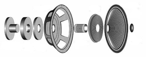
Let's attach to a cylindrical magnet surrounded by a coil a rigid structure that we call basket. Let us now stretch a diaphragm of low mass between the coil and the basket, the attachment being elastic, equivalent to a spring.
When the coil vibrates around its equilibrium position under the effect of the Laplace force (see below), it drags the diaphragm in its movement. The latter, in turn, causes the air to vibrate according to its radiation factor.
We will consider throughout this article that the speaker is mounted on an infinite baffle (see the previous article for the description of the model).

Set of parameters
A speaker is described by a set of mechanical and electrical parameters called Thiele and Small parameters. In order to illustrate the different results we will obtain, we choose here a Monacor SP-165PA entry-level woofer with a diameter of 16 cm, for which we give the catalog data.

- Effective membrane area S = 137\times10^{-4}\,\text{m}^2
- Mass of the moving part (coil + membrane) m = 8,2\times10^{-3} \,\text{kg})
- Stiffness of the elastic suspension k = 4,0\times 10^{3} \,\text{N}\,\text{m}^{-1}) (its inverse, compliance, is frequently found C = 1/k in units of \text{m}\,\text{N}^{-1})
- Mechanical resistance of the suspension \alpha= 1,2 \,\text{kg}\,\text{s}^{-1} (coefficient of the velocity in the expression of the drag)
- Coil's resistance R_e = 6.9\,\Omega (the index e refers to electrical quantities)
- Coil's inductance L_e= 0,50 \times10^{-3} \,\text{H}
- Force factor Bl = 7,1 \,\text{T}\,\text{m} (product of the magnetic field strength by the length of the coiled wire)
To which we add the limit value of the diaphragm excursion for which the response is linear: x_\text{max} = 3,75 \times10^{-3} \,\text{m}
Mechanical equation
Lorentz force
A charged particle, of charge q, in an electric field \vec{E} undergoes the electric force \vec{F_e}=q \cdot \vec{E}. This force is collinear to the electric field and has its direction if the particle is positively charged.
A charged particle, of charge q in motion at velocity \vec{v} is evolving in a magnetic field \vec{B}. It then undergoes the magnetic force \vec{F_m}=q\vec{v} \land \vec{B}, where the symbol \land stands for the cross product. The resulting direction of \vec{F_m} is found using the right hand rule (see figure).

Adding up these two forces, we get the Lorentz force qui s’exerce sur une particule chargée plongée dans un champ électromagnétique :
\vec{F}=q \cdot (\,\vec{E} + \vec{v} \land \vec{B})\,
Laplace force exerted on a conductor
Consider a wire-shaped electrical circuit, through which a current Iflows, in motion in an electromagnetic field (\, \vec{E},\,\vec{B} )\, at velocity \vec{V}.
All charged particles in the conductor (metal ions and free electrons) are subject to the Lorentz force.
For the metal ions, of positive charge, e standing for the elementary charge:
\vec{F}_{ion}=e \cdot (\,\vec{E} + \vec{V} \land \vec{B})\,
For free electrons, of opposite charge moving at speed \vec{u} in the circuit:
\vec{F}_{elec}=-e \cdot (\,\vec{E} + (\,\vec{V} + \vec{u})\,\land \vec{B})\,
There are as many metal ions as free electrons. All the contributions cancel out except the one due to the electrons' own speed in the circuit. The force exerted globally on the circuit, called Laplace force, is thus the sum of all \vec{f}=-e \vec{u}\land \vec{B} exerted upon each of the free electrons.
Special case of a speaker's coil
To simplify the following, let's place ourselves in the geometry that interests us for the study of the loudspeaker. The conductor is a coil of wire of total length l immersed in a radial magnetic field of intensity B :


According to the right hand rule, for a current flowing clockwise (and thus electrons flowing counterclockwise) all the forces to be summed are therefore collinear to the central axis of the device, directed along the increasing x . This is the convention chosen on the loudspeakers: the terminal tinted red or marked "+" corresponds to the direction of connection for which a positive current sets the moving equipment in motion towards the exterior. We still have to add up the contributions \vec{f}=-e\cdot u\cdot B \cdot \vec{e}_x for each free electrons (\vec{e}_x est le vecteur unitaire portant l’axe x).
How many free electrons are there in this coil? The current being the flow of charges, there are n=I/e electrons that cross a section of the circuit in one second. The last ones to cross it are those which were located at a distance \delta = u \times 1\,\text{s} one second before. If l is the length of the wire, there are therefore \frac{l}{\delta} times more : there is a total of N = n \cdot \frac{l}{\delta}=\frac{I \cdot l}{u\cdot e} free electrons. The Laplace force exerted on the coil is finally :
\vec{F}_L=N \cdot \vec{f}=\frac{I \cdot l}{u\cdot e} \cdot (\,-e)\,\cdot u\cdot B \cdot \vec{e}_x=I \cdot Bl \cdot \vec{e}_x
If the coil is traversed by a current of constant intensity i, the Laplace force exerted on it will therefore also be constant. But if we impose a variable current i in the coil, we see that the Laplace force will also be variable. It will push the coil sometimes to the right (when the current is positive) and sometimes to the left (when it is negative). The effect will be to make the coil vibrate around its equilibrium position.
The mechanical vibratory energy can then be transmitted in part to the air, as we have detailed in the previous article.
Finally, note that the Laplace force is proportional to the force factor Bl we can find on the speaker's specs.
Fundamental principle of dynamics
Let us apply the fundamental principle of dynamics to the system {coil + membrane} of mass m dans le référentiel de l’aimant : m \cdot \vec{a} = \Sigma\, \vec{F}_\text{ext}.
The forces exerted along the x axis are:
- the return force -k\cdot x due to the elastic fixation, which brings the system back to its equilibrium position;
- a dissipative force of fluid friction proportional to the speed of the system -\alpha \cdot v_x = -\alpha \cdot \dot{x} ;
- the Laplace force Bl \cdot i exerted on the coil ;
- the pressure forces -p_\text{avant} S and p_\text{arrière} S due to the pressure of the air on the faces of the membrane. These forces characterize the acoustic radiation of the loudspeaker.
We saw that the pressure forces were written: Z_\text{R} \cdot \dot{x}, with Z_\text{R} = R_\text{R} + j \omega m_\text{R} the radiation impedance. The expressions of the radiation resistance R_\text{R} and the radiation mass m_\text{R} are, for a piston embedded in an infinite plane, in the low frequency approximation :
\displaystyle{ R_\text{R} \approx \rho c S \sigma = \frac{\rho_0 S^2 }{2\pi c}\omega^2 \hspace{1cm}\text{et} \hspace{1cm} m_\text{R} \approx \frac{8\rho}{3}\left(\frac{S}{\pi}\right)^{3/2} }
For the Monacor speaker taken as an example, we get:
\displaystyle{ R_\text{R} \approx 1,0\times10^{-7}\omega^2 \;\text{kg}\,\text{s}^{-1}\hspace{1cm}\text{et} \hspace{1cm} m_\text{R} \approx 0,9 \,\text{g} }
The radiation resistance is therefore negligible compared to the mechanical resistance up to \omega \approx 10^3 \,\text{rad}\,\text{s}^{-1}. The expression used is in any case only valid at low frequencies. The radiation mass implies a small correction of a few percent.
In contrast to the solid piston model, the loudspeaker diaphragm is in contact with the air on both sides of the baffle: radiation mass and radiation resistance must be taken into account for the front radiation and for the back radiation.
We thus obtain the differential equation for the position of the coil (mechanical equation of the speaker:
(m + 2m_\text{R}) \cdot \ddot{x} = -k \cdot x - (\alpha + 2R_\text{R})\cdot \dot{x} + Bl \cdot i
Electrical equation
Induced electromotive force
When a circuit is mobile in a magnetic field, the magnetic force exerted on the free electrons will set them in motion. An induced current therefore appears spontaneously in the circuit. We call electromotive force u_\text{ind} the potential difference explaining the appearance of this electric current. We will establish in this paragraph the expression of the e.m.f. induced in the coil of a loudspeaker moving in the magnetic field of the magnet.
In the reference frame of the magnet, there is in the gap a radial magnetic field \vec{B} . When the coil is moving at the speed \vec{V}, the free electrons undergo a Lorentz force \vec{F}=-e \cdot \vec{V} \land \vec{B}. According to the right hand rule, this force will tend to set the electrons in motion in the trigonometric direction, and thus generate a positive current in the coil. By calling \vec{u} the unit vector directed at each point of the coil in the direction of a positive intensity : \vec{F}= e \cdot V \cdot B \cdot \vec{u}.
Let's place ourselves now in the reference frame of the coil. We have just seen that electrons initially at rest will start moving clockwise. They are thus subjected to the effect of an electric field \vec{E}' which is written, by definition :
\displaystyle{ \vec{E}' = \frac{\vec{F}}{q} = \frac{e \cdot V \cdot B \cdot \vec{u}}{-e}= V \cdot B \cdot \vec{u} }
The induced electromotive force is equal to the electric field circulation between the two ends of the coil;
u_\text{ind}= \int_0^l \vec{E}' \cdot \text d \vec{l} =- V \cdot Bl
Mesh equation
The mesh equation yields:
u(t)\, + u_\text{ind}(t)\, = u_R + u_L \, \iff \, R \cdot i + L \cdot \frac{\text{d}i}{\text{dt}} = u(t)\, - Bl \cdot \dot{x}
This equation is called electrical equation of the speaker. It is therefore, unsurprisingly, the equation of a steady state R,L circuit. But the voltage forcing the circuit contains two terms: the imposed voltage and the e.m.f. due to the speed of the coil.
Impedance
Sinusoidal steady state solutions
We have seen that the radiation resistance is small compared to the mechanical friction coefficient: R_\text{R} \ll \alpha. We will thus neglect the term containing R_\text{R} in this section which only deals with the electrical behavior of the loudspeaker.
A speaker is therefore governed by two equations:
\left\{ \begin{array}{ll} (m + 2m_\text{R})\cdot \ddot{x} + \alpha \cdot \dot{x} + k \cdot x = Bl \cdot i \\ R \cdot i + L \cdot \frac{\text{d}i}{\text{dt}} = u(\,t)\, - Bl\cdot \dot{x} \end{array}\right.
These equations are coupled, since the mechanical equation contains the electrical variable i and the electrical equation contains the mechanical variable x. The coupling coefficients are respectively Bl and - Bl : they are opposed to one another.
Let us look for particular solutions of these equations by imposing a sinusoidal regime. A more complex sound will be described by a set of frequencies, and thus by a sum of sinusoids, as explained here. Let's impose in the mechanical equation a sinusoidal intensity \underline{i}=\underline{I} \cdot \exp{(\,j \omega t)\,}. We use here the complex notation.
Let us now inject into the equation a sinusoidal solution for xi.e. a solution written as \underline{x}=\underline{X} \cdot \exp{(\,j \omega t)\,}. We get:
\left[(m + 2m_\text{R}) (j \omega)^2 + j \omega \alpha + k \right] \cdot \underline{X} = Bl \cdot \underline{I}
Operating in the same way for the electrical equation :
\underline{U} - Bl \cdot \underline{\dot{X}}= \left( R + j \omega L \right) \underline{I}
Eliminate \underline{X} of the second equation using the first :
\displaystyle{\underline{\dot{X}} = \frac{ j \omega \cdot Bl}{(m + 2m_\text{R}) (j\omega)^2 +j \omega \alpha + k} \cdot \underline{I}}
\displaystyle{\underline{U} = \left( R + j \omega L + \frac{j \cdot \omega \cdot (Bl)^2}{(m + 2m_\text{R}) (j\omega) ^2 +j \omega \alpha + k}\right)\underline{I}}
Where theimpedance of the speaker \underline{Z} = \underline{U} / \underline{I} appears:
\displaystyle{\underline{Z} = R + j \omega L + \frac{j \omega \cdot (Bl)^2}{(m + 2m_\text{R}) (j\omega)^2 -j \omega \alpha + k} }
The term R + j \omega L is the classical electrical impedance of a coil, the second term is due to the movement of the coil in the magnetic field of the magnet and is called motional impedance: :
\displaystyle{\underline{Z}_{\text{mot}} = \frac{j \omega \cdot l^2 \cdot B^2}{(m + 2m_\text{R}) \omega ^2 -j \omega \alpha - k} }
Equivalent electrical circuit
Note now that the motional impedance can be written :
\displaystyle{\underline{Z}_{\text{mot}} = \frac{1}{\frac{j \omega (m + 2m_\text{R})}{(Bl)^2} + \frac{\alpha}{(Bl)^2} +\frac{k}{j \omega (Bl)^2}} }
That is:
\displaystyle{\frac{1}{\underline{Z}_{\text{mot}}} = \frac{1}{j \omega L_\text{mot}}+ \frac{1}{R_\text{mot}} + \frac{1}{\frac{1}{j\omega C_\text{mot}} } }
with
\displaystyle{\left\{ \begin{array}{ll} L_{\text{mot}} = \frac{m + 2m_\text{R}}{(Bl)^2}\\ R_{\text{mot}} = \frac{(Bl)^2}{\alpha} \\ C_{\text{mot}} = \frac{(Bl)^2}{k} \end{array}\right.}
We thus recognize the association in parallel of a capacitor of capacity C_{\text{mot}}a resistor of resistance R_{\text{mot}} and a coil of inductance L_{\text{mot}}.
For the speaker used as an example, we obtain :
- C_{\text{mot}} = 198 \,\text{µF}
- R_\text{mot} = 42,0 \,\Omega
- L_\text{mot}= 12,6 \,\text{mH}
Let's take a moment to understand the physical origin of these three effects. The moving mass allows the storage of energy (due to inertia) like a coil stores magnetic energy when charged particles moves accross it. Friction forces dissipate energy as does a resistance by Joule effect. Finally, the stiffness of the spring allows, by the return force, the storage of elastic energy, as a capacitor stores electrical energy by adding up charges on both plates.
The equivalent electrical diagram of a loudspeaker is finally :

The resonance of the motional circuit R_{\text{mot}}, \, L_{\text{mot}} , \, C_{\text{mot}} in parallel occurs at the pulse
\displaystyle{\left( \frac{\text{d}\underline{Z}_\text{mot}}{\text{d}\omega}\right)_{\omega=\omega_0} = 0 \iff \omega_0 = \frac{1}{\sqrt{L_{\text{mot}} \cdot C_{\text{mot}}}} = \sqrt{\frac{k}{m + 2m_\text{R}}}}.

In our example, \omega_0 = 606\,\text{rad}\,\text{s}^{-1} that is f_0 = 96\,\text{Hz}. The peak of the impedance modulus is |\underline{Z}|_\text{max}=R_e+R_\text{mot}=49\,\Omega.
Two important facts to note here:
- The impedance peak at the resonance frequency f_0 = \frac{\omega_0}{2\pi} implies that the speaker cannot generate sound at a lower frequency. This frequency is therefore the low limit of the bandwidth. In fact, although it is marketed by displaying its power, an amplifier is indeed an amplifier of voltage. But the power is \mathcal{P} = \frac{U^2}{|\underline{Z}|}: it collapses when the frequency gets close to the impedance peak's.
- At low frequencies, the electrical impedance of the speaker is almost resistive: \underline{Z}_{e} = R_e + j\omega L_e \approx R_e. But when the pulsation approaches the value \omega = R_e/L_e (in our example, close to 14 000 \,\text{rad}\,\text{s}^{-1}), the inductive effects start to appear and the impedance rises.
- Between those two values, the modulus of the impedance passes through a minimum Zwhich is the impedance displayed by the manufacturer.
Only the acoustic performance of a speaker is, in fineof interest. The electrical study has however of interest that the measurement of the impedance curve, simpler to realize with precision than an acoustic measurement, allows to determine certain acoustic characteristics of the loudspeaker (motional resistance, resonance pulsation).
Acoustic radiation
Equivalent acoustical circuit
Let's start again from the mechanical equation and the electrical equation and eliminate the current from the mechanical equation. We obtain without difficulty :
\displaystyle{\frac{Bl\cdot\underline{U}}{R_e+j\omega L_e} = \left[ j\omega (m+2m_\text{R}) + (\alpha + 2R_\text{R}) + \frac{k}{j\omega} + \frac{(Bl)^2}{R_e + j\omega L_e} \right] \cdot \underline{\dot{X}} }
It is an equality between terms of the dimension of a force, i.e. energy per unit length. By dividing by the surface of the speaker S, we therefore obtain an equality between pressures (the Pascal is an energy per unit of volume):
\displaystyle{ \frac{(Bl)\cdot\underline{U}}{S(R_e+j\omega L_e)} = \left[ \frac{ j\omega (m+2m_\text{R})}{S^2} + \frac{\alpha + 2R_\text{R}}{S^2} + \frac{k}{j\omega S^2} + \frac{(Bl)^2}{S^2(R_e + j\omega L_e)} \right] \cdot \underline{Q}}where \underline{q} = S \cdot \dot{\underline{x}} = \underline{Q} \exp{(j \omega t)} is the acoustic flow of the speaker.
At low frequencies (\omega \ll R_e/L_e), the left-hand term is independent of the frequency:
\displaystyle{ \frac{(Bl)\cdot\underline{U}}{S\cdot R_e} = \left[ j\omega \frac{m + 2m_\text{R}}{S^2} + \frac{\alpha + 2R_\text{R}}{S^2} + \frac{1}{j\omega} \frac{k}{S^2} + \frac{(Bl)^2}{S^2\cdot R_e} \right] \cdot \underline{Q}}We then obtain an "electrical" equation describing a series association of four resistors, a capacitor and a coil:
\displaystyle{ \underline{P}_g = \left(R_{ae} + R_{as} + \frac{1}{j\omega \, C_{as}} + j\omega M_{as}+R_{ar,1}+R_{ar,2} \right) \cdot \underline{Q}}
With:
- The equivalent of the voltage is the excitation pressure \underline{p}_g=\underline{P}_g \exp (j\omega t) with \underline{P}_g = \frac{(Bl)\cdot\underline{U}}{S\cdot R_e}, in units of Pascals.
- The corresponding current is the acoustic flow (or volume velocity) \underline{q} = \underline{Q} \exp (j\omega t), in \text{m}^3/\text{s}
- The acoustic resistances are, in \text{Pa}\cdot\text{s}/\text{m}^3:
- R_{ae}=\frac{(Bl)^2}{S^2 R_e} (electrical losses in the coil)
- R_{as}=\frac{\alpha}{S^2} (frictional losses)
- The acoustic compliance (equivalent of a capacity) is, in \text{m}^3/\text{Pa} : C_{as}=\frac{S^2}{k}. The compliance, widely used in acoustics, is the opposite of the stiffness.
- The acoustic mass (equivalent of an inductance) is, in \text{kg}/\text{m}^4 : M_{as}=\frac{m + 2m_\text{R}}{S^2}
- The front and back radiation acoustic resistances R_{ar,1}=\frac{R_\text{R}}{S^2} and R_{ar,2}= R_{ar,1}
The index s following the 'acoustic' index a correspond to the speaker (speaker) alone. We will change it for a b (box) when it is mounted in a case and the corresponding quantities are changed.
We can now solve the physical problem by analogy with an electrical circuit. The equivalent circuit is as follows:

Acoustic flow
Here too, given the low efficiency of the speakers, we can neglect the radiation resistances in the calculation of the speaker output. The transfer function of the loudspeaker is then written :
\displaystyle{ \underline{Q} = \frac{1}{R_{ae} + R_{as} + \frac{1}{j\omega \, C_{as}} + j\omega M_{as}}\cdot \underline{P}_g }
\displaystyle{ \iff \underline{Q} = \frac{1}{( j\omega)^2 C_{as} M_{as} + j \omega C_{as}R_{ae} + j \omega C_{as}R_{as} + 1} \cdot j \omega C_{as} \underline{P}_g }
It is the transfer function of an oscillator damped by the resistive terms, which therefore behaves like a bandpass filter. Its resonance pulsation is : \omega_s^2 = 1/(C_{as}M_{as}) = k/(m + 2m_\text{R}) = \omega_0^2. The resonance of the acoustic flow takes place at the frequency corresponding to the electrical impedance peak.
Let's call:
- \nu = \omega / \omega_s the reduced pulsation ;
- Q_{es} =\frac{1}{\omega_s C_{as}R_{ae}} the electrical quality factor (for the Moncaor Q_{es} = 1,11) ;
- Q_{ms} =\frac{1}{\omega_s C_{as}R_{as}} the mechanical quality factor (for the Monacor Q_{ms}= 5,0).
The expression of the acoustic flow becomes:
\displaystyle{ \underline{Q} = \frac{j\nu}{( j\nu)^2 + j\nu \left(\frac{1}{Q_{es}}+ \frac{1}{Q_{ms}}\right) + 1} \cdot \omega_s C_{as} \underline{P}_g }
Let's finally call Q_{ts} the total quality factor such that \frac{1}{Q_{ts}} = \frac{1}{Q_{es}} + \frac{1}{Q_{ms}} (in our example, we have Q_{ts} = 0,91 ):
\displaystyle{\boxed{ \underline{Q} = \frac{j\nu}{( j\nu)^2 +\frac{j\nu}{Q_{ts}} + 1} \cdot \omega_s C_{as} \underline{P}_g }}Radiated power
We know that:
\displaystyle{ \mathcal{P}_{ar} = R_\text{R} V_\text{eff}^2 = \frac{R_\text{R}}{S^2} Q_\text{eff}^2 = \frac{R_\text{R}}{2 S^2} |Q|^2}
Furthermore R_\text{R} = \rho_0 c S \sigma. We get:
\displaystyle{ \mathcal{P}_{ar} = \frac{\rho_0 c \sigma}{2 S} |Q|^2}
We are here in low frequency approximation with respect to the characteristics of the speaker (\omega \ll \frac{R_e}{L_e}). The low frequencies with respect to the acoustic characteristics are defined by ka \ll 1 \iff \omega \ll \frac{c}{a} (a being the radius of the membrane).
In our example, we have a = \sqrt{S/\pi} = 0,066 \, \text{m} : \omega \ll \frac{c}{a} \approx 5 000 \, \text{rad}\cdot \text s ^{-1} \approx 800 \, \text{Hz}
These two approximations are therefore of the same order of magnitude. In their respect ( f < 300 \, \text{Hz}), the radiation factor of the baffled speaker is, as already used above, \sigma \approx \frac{a^2 k^2}{2} = \frac{S}{2\pi c^2}\omega^2. We get:
\displaystyle{ \mathcal{P}_{ar} = \frac{\rho_0 }{4\pi c}\omega^2|Q|^2 }
The response curve of the speaker at low frequencies is then, by injecting the expression of the acoustic flow's amplitude :
\displaystyle{ \boxed{ \mathcal{P}_{ar} = \frac{\rho_0 \left( \omega_s^2 C_{as} \underline{P}_g \right) ^2}{4\pi c} \left|\underline{H}_P\right|^2} \hspace{1cm} \text{avec} \hspace{1cm} \boxed{\underline{H}_P = \frac{\nu^2}{( j\nu)^2 +\frac{j\nu}{Q_{ts}} + 1} }}
On the form a+jb, the transfer function is written:
\displaystyle{ \underline{H}_P = \frac{ \displaystyle{\frac{\nu^3}{Q_{ts}}}+j \nu^2 (1-\nu^2)} {\nu^4 + \nu^2 \left(-2 + \displaystyle{\frac{1}{Q_{ts}^2}} \right) + 1} }
Its squared modulus is therefore:
\displaystyle{ |\underline{H}_P|^2 = \frac{\nu^4} {\nu^4 + \nu^2 \left(-2 + \displaystyle{\frac{1}{Q_{ts}^2}} \right) + 1} }
At low frequencies \nu \rightarrow 0, an expansion at first non-zero order yields |\underline{H}_P|^2 \approx \nu^4. The asymptotic behavior of the sound level is thus a straight line with a slope of 12 dB/octave (the power is indeed multiplied by 2^4=16 when the frequency doubles).
The square of the modulus of the transfer function is as follows:

We see on the previous expression that there will be a resonance (red and purple curves above) only if -2 + \frac{1}{Q_{ts}^2} < 0 \iff Q_{ts} > 1/\sqrt{2}. A good speaker will ensure a smooth transition to the bass and will therefore not have a pronounced power peak: it will have a maximum quality factor Q_{ts} \leq \frac{1}{\sqrt{2}}.
The cut-off at 3\,\text{dB} occurs when |\underline{H}_P|^2 = \frac{1}{2}, that is:
\nu_3^2 = \left( \frac{1}{2Q_{ts}^2}-1\right) + \sqrt{1+\left( \frac{1}{2Q_{ts}^2}-1\right)^2}
With numerical values:
- Q_{ts} = 0,3 \hspace{1cm} \nu_3 = 9.2
- Q_{ts} = 0,5 \hspace{1cm} \nu_3 = 2.4
- Q_{ts} = 0,7 \hspace{1cm} \nu_3 = 1,0
- Q_{ts} = 0,9 \hspace{1cm} \nu_3 = 0,7
- Q_{ts} = 1,2 \hspace{1cm} \nu_3 = 0,6
In order for it to provide maximum power until cut-off (as opposed to the blue and orange curves which collapse early), a good speaker will therefore have a total quality factor close to Q_{ts} \approx 1/\sqrt{2} \approx 0,7 (green curve).
The speaker we're studying, with Q_{ts} \approx 0,9is close to the red curve. From the point of view of the -3 dB cutoff in the bass, it is rather good. From the point of view of a smooth transition to the bass, it is not an excellent choice.
Efficiency
The efficiency of the speaker is:
\displaystyle{ \eta = \frac{\mathcal{P}_{ar}}{\mathcal{P}_e} }
where \mathcal{P}_e = \frac{U_\text{eff}^2}{|\underline{Z}|} is the electrical power consumed by the loudspeaker. As these quantities depend on the frequency, the efficiency will be evaluated at the minimum of the impedance module, for which |\underline{Z}| \approx R_e and |\underline{H}_P| = 1. We thus have:
\displaystyle{ \eta_0 = \frac{\rho_0}{4\pi c} \frac{ \left(\omega_s^2 C_{as} \underline{P}_g \right) ^2}{U_\text{eff}^2/R_e} }
Developing the expression of the excitation pressure, we get:
\displaystyle{ \eta_0 = \frac{\rho_0}{4\pi c} \frac{ \left(\omega_s^2 C_{as} \frac{(Bl)\sqrt{2}U_\text{eff}}{S\cdot R_e} \right) ^2}{U_\text{eff}^2/R_e} = \frac{\rho_0}{2\pi R_e c} \left( \frac{\omega_s^2 C_{as}(Bl)}{S} \right) ^2 }
That, in turns, becomes as a function of the speaker's parameters only:
\displaystyle{ \boxed{ \eta_0 = \frac{\rho_0}{2\pi R_e c} \left( \frac{S(Bl)}{m + 2m_\text{R}} \right) ^2 }}The numerical value for our example is: \eta_0 = 0,8\%.
The efficiency of a loudspeaker is generally less than 1%, which justifies in another way to have neglected in the previous calculations the radiation resistance.
Sound level, sensitivity
In the far field, the radiation from the diaphragm is isotropic. The sound intensity at a distance r is thus obtained by dividing the acoustic power by the surface of the half-sphere on which the energy is diluted:
I = \displaystyle{ \frac{\mathcal{P}_{ar}}{2\pi r^2} = \frac{\rho_0}{8\pi^2 c}\left(\frac{\omega_s^2 C_{as} \underline{P}_g}{r} \right)^2 \left| \underline{H}_P \right|^2 }
The sound level is, by definition:
L=10\, \log \frac{I}{I_0}
The sensitivity L_1 of a speaker is the sound level obtained at a distance of r_0 = 1 \,\text{m} from the loudspeaker when supplied with an RMS voltage U_\text{eff}= 2,83V (which, for an impedance of 8 \Omegacorresponds to an average electrical power \mathcal{P}_e = U_\text{eff}^2/Z=1\,\text{W}). The sensitivity is evaluated in the frequency range where the speaker is most effective (|\underline{H}_P| = 1).
Using this definition, we can write:
\displaystyle{ L_1=10\, \log \frac{\eta_0 U_\text{eff}^2 / (2\pi R_e)}{I_0}=10\, \log \frac{ U_\text{eff}^2}{2\pi I_0} + 10\, \log \frac{\eta_0}{R_e} = 121,1 + 10\, \log \frac{\eta_0}{R_e} }
This relationship yields, when applied to the woofer : L_1 = 91,5\,\text{dB}.
Displacement of the diaphragm
The excursion of the membrane \underline{x} = \underline{X} \exp (j \omega t) = \frac{\underline{V}}{j\omega} \exp (j\omega t) is obtained from the expression of the volume velocity:
\displaystyle{ \underline{X} = \frac{\underline{V}}{j \nu \omega_s} = \frac{\underline{Q}}{j \nu \omega_s S} = \frac{1}{j\nu \omega_s S} \frac{j\nu}{( j\nu)^2 +\frac{j\nu}{Q_{ts}} + 1} \cdot \omega_s C_{as} \underline{P}_g }
That is:
\displaystyle{ \underline{X} = \underline{H}_X \cdot \frac{C_{as} \underline{P}_g}{S} }
with \displaystyle{ \underline{H}_X = \frac{1}{( j\nu)^2 +\frac{j\nu}{Q_{ts}} + 1} }
whose modulus is \displaystyle{ |\underline{H}_X| = \frac{1}{\sqrt{\nu^4 +\nu^2\left(-2+\frac{1}{Q_{ts}^2}\right) + 1} } }
As for the power, there will be no resonance for a good loudspeaker with a total quality factor equal or very close to 1/\sqrt{2}. In this case, the maximum displacement is at \nu=0 :

Maximal values
Voltage and electrical power
The effective displacement of the loudspeaker depends on the voltage imposed by the amplifier (appearing in the expression of the excitation pressure \underline{P}_g). The maximum permissible voltage is therefore the voltage at which the loudspeaker reaches its maximum linear elongation x_\text{max}.
But at which frequency should we do this calculation?
- On the one hand, the displacement is maximal at low frequencies
- On the other hand, we have seen that the power collapses when attacking the impedance peak of the speaker.
We can then estimate the maximum voltage required by doing the calculation at half the peak of the motional impedance: we select \omega_p such that |\underline{Z_\text{mot}}|(\omega_p)=\frac{|\underline{Z}|_\text{mot,max}}{2}.

The expression of the motional impedance can be put in the form :
\displaystyle{ |Z_\text{mot,p}|^2=\left( \frac{R_\text{mot}}{2} \right)^2 = \frac{\omega_p^2 (Bl)^4}{(m + 2m_\text{R})^2\omega_p^4 + (\alpha^2 - 2 (m+2m_\text{R}) k) \omega_p^2 + k^2} }
The solution of the second degree equation in \omega_p^2 leads in our example to : f_p = 108 \,\text{Hz}.
The displacement of the membrane to be taken into account for this calculation is therefore :
\displaystyle{ |\underline{X}| = |\underline{H}_X(\omega_p)| \cdot \frac{C_{as} P_g} {S} }
Let us inject the expression of the excitation pressure and impose |\underline{X}|=x_\text{max}:
\displaystyle{ x_\text{max} = |\underline{H}_X(\omega_p)| \cdot \frac{C_{as} (Bl)\cdot U_\text{max}}{S^2\cdot R_e} = |\underline{H}_X(\omega_p)| \cdot \frac{(Bl)\cdot U_\text{max}}{k\cdot R_e} }We get:
\displaystyle{ U_\text{max} = \frac{1}{ |\underline{H}_X(\omega_p)| }\cdot \frac{k R_e x_\text{max}} {Bl} }
For the woofer we find U_\text{max}=22\,\text{V}. The maximum power required from the amplifier is then \mathcal{P}_{e,\text{max}} = \frac{U_\text{max}^2}{R_e}= 68\,\text W. The latter is calculated not at the impedance peak but at its minimum value \approx R_e. The speaker's datasheet indicates 50 \,\text W_\text{RMS} and 100 \,\text W at peak, but it corresponds only to electrical and not acoustic criteria.
Maximum sound level
We can now recalculate the sound level with the maximum peak voltage we just obtained:
\displaystyle{ L_\text{max}=10\, \log \frac{ U_\text{max}^2/2}{2\pi I_0} + 10\, \log \frac{\eta_0}{R_e} }For the Monacor Woofer, we get: L_\text{max}=112\,\text{dB}. As we will see in the next article, and as many other results obtained here, this value will be modified when placed in a box.
High frequencies
The radiated power was calculated in the low frequency approximation. We have indeed used an expansion of the radiation factor for ka \ll 1, which corresponds to a limit frequency for our example f \ll 830 \,\text{Hz}. Moreover, the radiation resistance at high frequencies is no longer negligible compared to the mechanical resistance. Finally, the low-frequency approximation results in the quasi-isotropic emission of the loudspeaker, and we have therefore neglected its directivity.
All the previous calculations are therefore valid, as we have already said, only for frequencies lower than a few hundred Hertz. But the loudspeaker that we study is announced to be able to emit from 93 Hz (its resonance frequency) to 5500 Hz.
Let's compare the model we have developed (in red) with the measured response curve of the speaker:

The blue vertical marker corresponds to ka=1, le repère vertical rouge correspond à la fréquence maximale d’utilisation indiquée par le fabricant.
The yellow line modeling the cutoff has a slope of 24 decibels per octave.
If the model explained in this article is very efficient to determine the properties of a loudspeaker at low frequencies, it is insufficient to characterize its high cutoff frequency and the sometimes pronounced "accidents" appearing on the response curve. For example, the SP-165PA shows a sudden drop in sound level around 1 kHz, then oscillations that appear around 5 kHz.
What can be predicted about the radiation of the speaker beyond the low frequency approximation? This will be the subject of a future article to provide some answers.
Conclusion
In this article, we have presented a model of the electro-dynamic speaker embedded in an infinite baffle, allowing to understand the phenomena at work behind the response curve and to calculate precisely this curve at low frequencies. The low frequency domain is particularly useful to predict the low cutoff frequency of the loudspeaker, the required electrical power, and the expected maximum sound level.
In the next article, we will see how these quantities are modified when the loudspeaker is embedded in a cabinet to make a loudspeaker.
Sources
José-Philippe Pérez – Mécanique (DUNOD)
Francis BROUCHIER – Haut-parleurs et enceintes acoustiques : Théorie et pratique
Jean Fourcade – Utilitaires Scilab pour le calcul et l’optimisation d’enceintes bass-reflex